Bayesian Golf Putting Model

Introduction

Disclaimer

This is inspired from Dr. Andrew Gelman’s case study, which can be found here. Specifically:

• This is heavily inspired by Colin Caroll’s Blog present here. A lot of the plotting code from his blog post has been reused.
• Josh Duncan’s blog post on the same topic which can be found here.

This is not a novel solution. It is merely a replication of Dr. Gelman’s blog in PyMC3.

Problem

This is based on a popular blog post by Dr. Andrew Gelman. Here, we are given data from professional golfers on the proportion of success putts from a number of tries. Our aim is to identify:

Can we model the probability of success in golf putting as a function of distance from the hole?

EDA

import pandas as pd
import numpy as np
import pymc3 as pm
import matplotlib.pyplot as plt
import seaborn as sns

WARNING (theano.tensor.blas): Using NumPy C-API based implementation for BLAS functions.

The source repository is present here

data = np.array([[2,1443,1346],
[3,694,577],
[4,455,337],
[5,353,208],
[6,272,149],
[7,256,136],
[8,240,111],
[9,217,69],
[10,200,67],
[11,237,75],
[12,202,52],
[13,192,46],
[14,174,54],
[15,167,28],
[16,201,27],
[17,195,31],
[18,191,33],
[19,147,20],
[20,152,24]])

df = pd.DataFrame(data, columns=[
    'distance', 
    'tries', 
    'success_count'
])

df

	distance	tries	success_count
0	2	1443	1346
1	3	694	577
2	4	455	337
3	5	353	208
4	6	272	149
5	7	256	136
6	8	240	111
7	9	217	69
8	10	200	67
9	11	237	75
10	12	202	52
11	13	192	46
12	14	174	54
13	15	167	28
14	16	201	27
15	17	195	31
16	18	191	33
17	19	147	20
18	20	152	24

The variables have the following format:

Variable	Units	Description
distance	feet	Distance from the hole for the putt attempt
tries	count	Number of attempts at the chosen distance
success_count	count	The total successful putts

Lets try to visualize the dataset:

df['success_prob'] = df.success_count / df.tries

sns.set()
plt.figure(figsize=(16, 6))
ax = sns.scatterplot(x='distance', y='success_prob', data=df, s=200)
ax.set(xlabel='Distance from hole(ft)', ylabel='Probability of Success')

[Text(0, 0.5, 'Probability of Success'),
 Text(0.5, 0, 'Distance from hole(ft)')]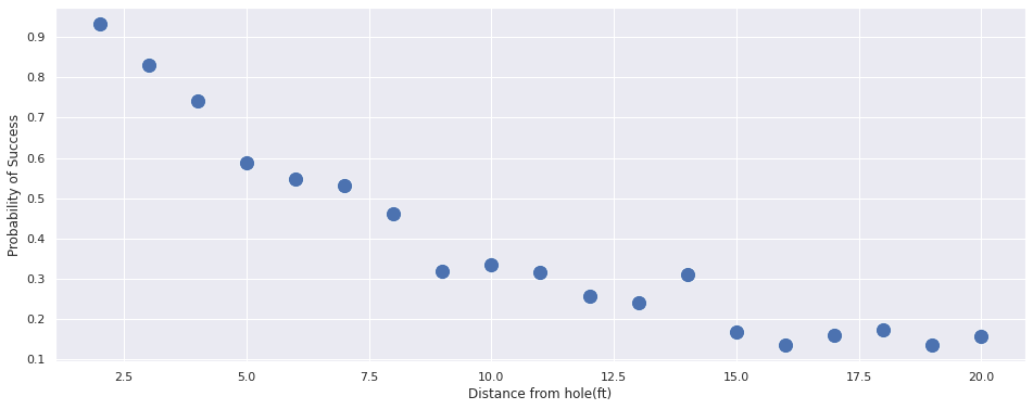

We can notice that the probability of success decreases as the distance increases.

Baseline Model

Let us try to see we can fit a simple linear model to the data i.e Logsitic Regression. We will be using PyMC3.

Here, we will attempt to model the success of golf putting by using the distance as an independant(i.e predictor) variable. The model will have the following form:

\[y_i \sim binomial(n_j, logit^{-1}(b_0 + b_1x_j)), \text{for } j = 1,...J \]

with pm.Model() as model:
    b_0 = pm.Normal('b_0', mu=0, sd=1)
    b_1 = pm.Normal('b_1', mu=0, sd=1)
        
    y = pm.Binomial(
        'y', 
        n=df.tries, 
        p=pm.math.invlogit(b_0 + b_1 * df.distance), 
        observed=df.success_count
    )

Why are we using inverse logit?

• Logit is a function used to convert a continous variable to a value in the range [0,1]
• Inverse Logit: Used to convert real valued variable to a value in the range [0,1]

pm.model_to_graphviz(model)

with model:
    trace = pm.sample(1000, tune=1000, chains=4)

Auto-assigning NUTS sampler...
Initializing NUTS using jitter+adapt_diag...
Multiprocess sampling (4 chains in 2 jobs)
NUTS: [b_1, b_0]
Sampling 4 chains, 0 divergences: 100%|██████████| 8000/8000 [00:06<00:00, 1164.22draws/s]
The acceptance probability does not match the target. It is 0.889539212527967, but should be close to 0.8. Try to increase the number of tuning steps.
The acceptance probability does not match the target. It is 0.6968711559119489, but should be close to 0.8. Try to increase the number of tuning steps.
The number of effective samples is smaller than 25% for some parameters.

pm.summary(trace)[['mean', 'sd', 'mcse_mean', 'mcse_sd', 'ess_mean', 'r_hat']]

	mean	sd	mcse_mean	mcse_sd	ess_mean	r_hat
b_0	2.226	0.060	0.002	0.001	926.0	1.01
b_1	-0.255	0.007	0.000	0.000	838.0	1.01

pm.traceplot(trace)

array([[<matplotlib.axes._subplots.AxesSubplot object at 0x7fdfef7cfd68>,
        <matplotlib.axes._subplots.AxesSubplot object at 0x7fdfef77efd0>],
       [<matplotlib.axes._subplots.AxesSubplot object at 0x7fdfef848828>,
        <matplotlib.axes._subplots.AxesSubplot object at 0x7fdfef758a58>]],
      dtype=object)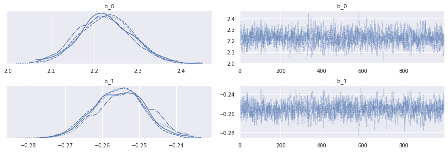

pm.plot_posterior(trace)

array([<matplotlib.axes._subplots.AxesSubplot object at 0x7fdfedd70be0>,
       <matplotlib.axes._subplots.AxesSubplot object at 0x7fdfedd2a860>],
      dtype=object)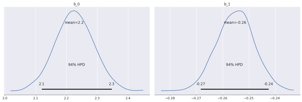

From the above results, we can see:

• PyMC3 has estimated
  • \(b_0\) to be \(2.23 \pm 0.057\)
  • \(b_1\) to be \(-0.26 \pm 0.007\)
• The MCSE is almost 0 \(\implies\) The simulation has run long enough for the chains to converge.
• \(r\_hat = 1.0\) tells us that the chains have mixed well i.e hairy hedgehog pattern.

Let us plot the final output of this model and check it with our training data.

with model:
    posterior_trace = pm.sample_posterior_predictive(trace)

100%|██████████| 4000/4000 [00:04<00:00, 888.12it/s]

posterior_success = posterior_trace['y'] / df.tries.values

df['posterior_success_prob'] = pd.DataFrame(posterior_success).median()
df['posterior_success_prob_std'] = pd.DataFrame(posterior_success).std()

sns.set()
plt.figure(figsize=(16, 6))
prob = df.success_count/df.tries
ax = sns.scatterplot(x='distance', y=df.success_prob, data=df, s=200, label='actual')
# ls = np.linspace(0, df.distance.max(), 200)
# for index in np.random.randint(0, len(trace), 50):
#     ax.plot(
#         ls, 
#         scipy.special.expit(
#             trace['b_0'][index] * ls + trace['b_1'][index] * ls
#         )
#     )
sns.scatterplot(x='distance', y=df.posterior_success_prob, data=df, label='predicted',ax=ax, color='red', s=200)
sns.lineplot(x='distance', y=df.posterior_success_prob, data=df,ax=ax, color='red')
ax.set(xlabel='Distance from hole(ft)', ylabel='Probability of Success')

[Text(0, 0.5, 'Probability of Success'),
 Text(0.5, 0, 'Distance from hole(ft)')]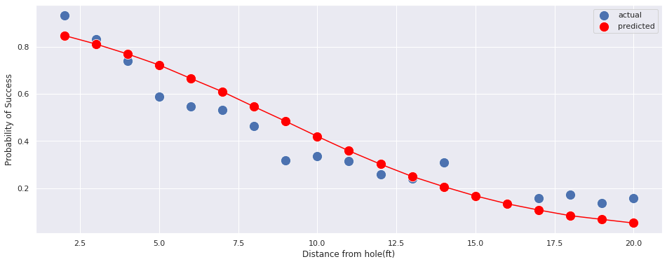

The curve fit is okay, but it can be improved. We can use this as a baseline model. In reality, each of them is not a point, but an posterior estimate. Because the uncertainity is small(as seen above), we’ve decided to show only the median points.

From the above model, putts from 50ft are expected to be made with probability:

import scipy
res = 100 * scipy.special.expit(2.223 + -0.255 * 50).mean()
print(np.round(res, 5),"%")

0.00268 %

Modelling from first principles

Geometry based Model

We’ll try to accomodate the physics associated with the problem. Specically, we assume:

Assumptions

• The golfers can hit the ball in any direction with some small error. This error could be because of inaccuracy, errors in the human, etc.
• This error refers to the angle of the shot.
• We assume the angle is normally distributed.

Implications

• The ball goes in whenever the angle is small enough for it to hit the cup of the hole!
• Longer putt \(\implies\) Larger error \(\implies\) Lower success rate than shorter putt

From Dr. Gelman’s blog, we obtain the formula as:

\(Pr(|angle| < sin^{-1}(\frac{(R-r)}{x})) = 2\phi\big(\frac{sin^{-1}\frac{R-r}{x}}{\sigma}\big) - 1\)

\(\phi \implies\) Cumulative Normal Distribution Function.

Hence, our model will now have two big parts:

\[y_j \sim binomial(n_j, p_j)\]

\[p_j = 2\phi\big(\frac{sin^{-1}\frac{R-r}{x}}{\sigma}\big) - 1\]

Typically, the diameter of a golf ball is 1.68 inches and the cup is 4.25 inches i.e

\[r = 1.68 \text{inch}\] \[R = 4.25 \text{inch}\]

ball_radius = (1.68/2)/12
cup_radius = (4.25/2)/12

def calculate_prob(angle, distance):
    """
    Calculate probability that the ball with fall in the hole given the angle of the shot 
    and the distance from the hole.
    """
    rad = angle * np.pi / 180.0
    arcsin = np.arcsin((cup_radius - ball_radius)/ distance)
    return 2 * scipy.stats.norm(0, rad).cdf(arcsin) - 1

plt.figure(figsize=(16, 6))
ls = np.linspace(0, df.distance.max(), 200)
ax = sns.scatterplot(
    x='distance', 
    y='success_prob', 
    data=df, 
    s=100,
    legend='full'
)
for angle in [0.5, 1, 2, 5, 20]:
    ax.plot(
        ls, 
        calculate_prob(angle, ls), 
        label=f"Angle={angle}"
    )
ax.set(
    xlabel='Distance from hole(ft)', 
    ylabel='Probability of Success'
)
ax.legend()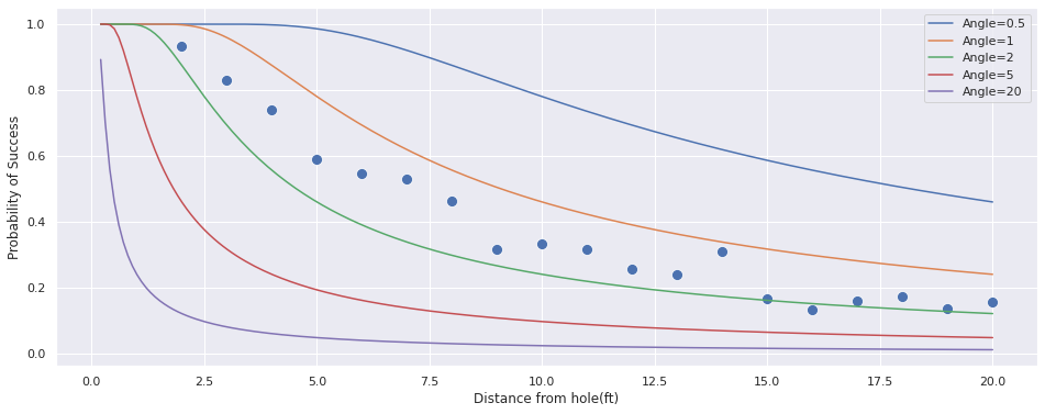

Let us now add this to our model!

import theano.tensor as tt


def calculate_phi(num):
    "cdf for standard normal"
    q = tt.erf(num / tt.sqrt(2.0)) # ERF is the Gaussian Error 
    return (1.0 + q) / 2.

with pm.Model() as model:
    angle_of_shot_radians = pm.HalfNormal('angle_of_shot_radians')
    angle_of_shot_degrees = pm.Deterministic(
        'angle_of_shot_degrees',
        (angle_of_shot_radians * 180.0) / np.pi
    )
    p_ball_goes_in = pm.Deterministic(
        'p_ball_goes_in',
        2 * calculate_phi(
                tt.arcsin(
                    (cup_radius - ball_radius)/ df.distance
                ) / angle_of_shot_radians
            )
        ) - 1
    p_success = pm.Binomial(
        'p_success',
        n=df.tries, 
        p=p_ball_goes_in, 
        observed=df.success_count
    )

pm.model_to_graphviz(model)

with model:
    trace = pm.sample(4000, tune=1000, chains=4)

Auto-assigning NUTS sampler...
Initializing NUTS using jitter+adapt_diag...
ERROR (theano.gof.opt): Optimization failure due to: local_grad_log_erfc_neg
ERROR (theano.gof.opt): node: Elemwise{true_div}(Elemwise{mul,no_inplace}.0, Elemwise{erfc,no_inplace}.0)
ERROR (theano.gof.opt): TRACEBACK:
ERROR (theano.gof.opt): Traceback (most recent call last):
  File "/home/goodhamgupta/shubham/blog/_notebooks/.env/lib/python3.6/site-packages/theano/gof/opt.py", line 2034, in process_node
    replacements = lopt.transform(node)
  File "/home/goodhamgupta/shubham/blog/_notebooks/.env/lib/python3.6/site-packages/theano/tensor/opt.py", line 6789, in local_grad_log_erfc_neg
    if not exp.owner.inputs[0].owner:
AttributeError: 'NoneType' object has no attribute 'owner'

Multiprocess sampling (4 chains in 2 jobs)
NUTS: [angle_of_shot_radians]
Sampling 4 chains, 0 divergences: 100%|██████████| 20000/20000 [00:10<00:00, 1943.54draws/s]
The acceptance probability does not match the target. It is 0.8844154441842546, but should be close to 0.8. Try to increase the number of tuning steps.

pm.summary(trace).head(2)

	mean	sd	hpd_3%	hpd_97%	mcse_mean	mcse_sd	ess_mean	ess_sd	ess_bulk	ess_tail	r_hat
angle_of_shot_radians	0.027	0.000	0.026	0.027	0.0	0.0	6641.0	6641.0	6641.0	10874.0	1.0
angle_of_shot_degrees	1.527	0.023	1.484	1.570	0.0	0.0	6641.0	6641.0	6641.0	10874.0	1.0

pm.plot_posterior(trace['angle_of_shot_degrees'])

array([<matplotlib.axes._subplots.AxesSubplot object at 0x7fdfe4c24f60>],
      dtype=object)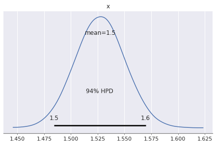

From the above results, we can see:

• PyMC3 has estimated
  • \(angle_of_shot_degrees\) to be \(1.53 \pm 0.023\)
• The MCSE is almost 0 \(\implies\) The simulation has run long enough for the chains to converge.
• \(r\_hat = 1.0\) tells us that the chains have mixed well i.e hairy hedgehog pattern.

Let’s visualize the fit with this new model:

geo_model_prob = calculate_prob(
    trace['angle_of_shot_degrees'].mean(), 
    df.distance
)

sns.set()
plt.figure(figsize=(16, 6))

ax = sns.scatterplot(x='distance', y=df.success_prob, data=df, s=200, label='Actual')

sns.scatterplot(x='distance', y=df.posterior_success_prob, data=df, label='Logistic Regression',ax=ax, color='red', s=100)
sns.scatterplot(x='distance', y=geo_model_prob, data=df, label='Geometry based ',ax=ax, color='orange', s=100)

sns.lineplot(x='distance', y=df.posterior_success_prob, data=df,ax=ax, color='red')
sns.lineplot(x='distance', y=geo_model_prob, data=df,ax=ax, color='orange')

ax.set(xlabel='Distance from hole(ft)', ylabel='Probability of Success')

[Text(0, 0.5, 'Probability of Success'),
 Text(0.5, 0, 'Distance from hole(ft)')]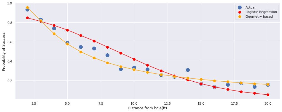

• We can see that the geometry based model fits better than the logistic regression model.
• While this model is not completely accurate, it suggests that angle is a good variable to model the problem. Using this model, we can be more confident about extrapolating the data.
• For the same 50ft putt, the probability now is:

import scipy
lr_result = np.round(
    100 * scipy.special.expit(2.223 + -0.255 * 50).mean(),
    5
)
geo_result = np.round(
    100 * calculate_prob(
        trace['angle_of_shot_degrees'].mean(), 
        50
    ).mean(),
    5
)

print(
    f"Logistic Regression Model: {lr_result}% \n"\
    f"Geometry Based Model: {geo_result}%"
)

Logistic Regression Model: 0.00268% 
Geometry Based Model: 6.40322%

New Data!

Mark Broadie obtained new data about the golfers. Let’s see how our model performs on this new dataset.

First, we’ll look at the summary of the dataset.

#  golf putting data from Broadie (2018)
new_golf_data = np.array([
[0.28, 45198, 45183],
[0.97, 183020, 182899],
[1.93, 169503, 168594],
[2.92, 113094, 108953],
[3.93, 73855, 64740],
[4.94, 53659, 41106],
[5.94, 42991, 28205],
[6.95, 37050, 21334],
[7.95, 33275, 16615],
[8.95, 30836, 13503],
[9.95, 28637, 11060],
[10.95, 26239, 9032],
[11.95, 24636, 7687],
[12.95, 22876, 6432],
[14.43, 41267, 9813],
[16.43, 35712, 7196],
[18.44, 31573, 5290],
[20.44, 28280, 4086],
[21.95, 13238, 1642],
[24.39, 46570, 4767],
[28.40, 38422, 2980],
[32.39, 31641, 1996],
[36.39, 25604, 1327],
[40.37, 20366, 834],
[44.38, 15977, 559],
[48.37, 11770, 311],
[52.36, 8708, 231],
[57.25, 8878, 204],
[63.23, 5492, 103],
[69.18, 3087, 35],
[75.19, 1742, 24],
])

new_df = pd.DataFrame(
    new_golf_data, 
    columns=['distance', 'tries', 'success_count']
)

new_geo_model_prob = calculate_prob(
    trace['angle_of_shot_degrees'].mean(), 
    new_df.distance
)

new_df['success_prob'] = new_df.success_count / new_df.tries
sns.set()
plt.figure(figsize=(16, 6))
ax = sns.scatterplot(x='distance', y='success_prob', data=df, label='Old Dataset', s=200)
sns.scatterplot(x='distance', y='success_prob', data=new_df,label='New Dataset', s=200, ax=ax)
sns.scatterplot(x='distance', y=new_geo_model_prob, data=new_df, label='Geometry based Model ',ax=ax, color='red', s=100)
ax.set(
    xlabel='Distance from hole(ft)', 
    ylabel='Probability of Success'
)
plt.setp(ax.get_legend().get_texts(), fontsize='25')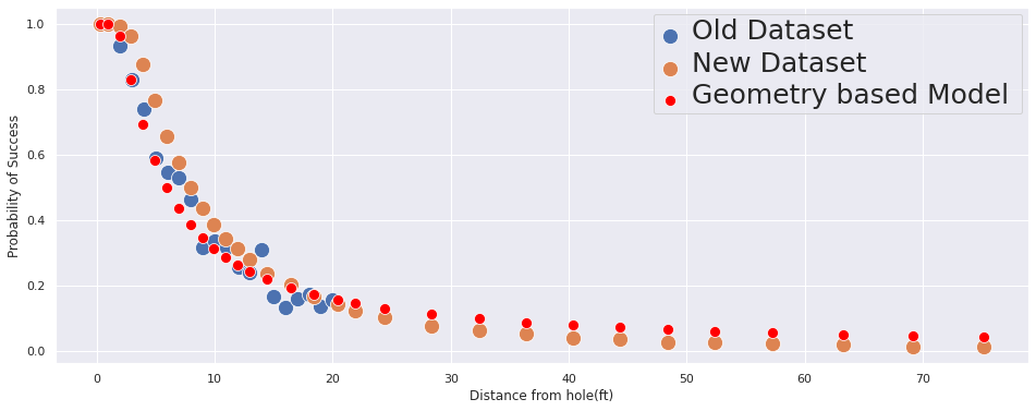

We can see:

• Success rate is similar in the 0-20 feet range for both datasets.
• Beyond 20 ft, success rate is lower than expected. These attempts are more difficult, even after we have accounted for increased angular precision.

Moar features!

To get the ball in, along with the angle, we should also need to take into account if the ball was hit hard enough.

From Colin Caroll’s Blog, we have the following: > Mark Broadie made the following assumptions - If a putt goes short or more than 3 feet past the hole, it will not go in. - Golfers aim for 1 foot past the hole - The distance the ball goes, \(u\), is distributed as: \[ u \sim \mathcal{N}\left(1 + \text{distance}, \sigma_{\text{distance}} (1 + \text{distance})\right), \] where we will learn \(\sigma_{\text{distance}}\).

After working through the geometry and algebra, we get:

\[P(\text{Good shot}) = \bigg(2\phi\big(\frac{sin^{-1}(\frac{R-r}{x})}{\sigma_{angle}}\big)-1\bigg)\bigg(\phi\bigg(\frac{2}{(x+1)\sigma_{distance}}\bigg) - \phi\bigg(\frac{-1}{(x+1)\sigma_{distance}}\bigg)\bigg)\]

Let’s write this down in PyMC3

OVERSHOT = 1.0
DISTANCE_TOLERANCE = 3.0
distances = new_df.distance.values
with pm.Model() as model:
    angle_of_shot_radians = pm.HalfNormal('angle_of_shot_radians')
    angle_of_shot_degrees = pm.Deterministic(
        'angle_of_shot_degrees',
        (angle_of_shot_radians * 180.0) / np.pi
    )
    
    variance_of_distance = pm.HalfNormal('variance_of_distance')
    p_good_angle = pm.Deterministic(
        'p_good_angle',
        2 * calculate_phi(
                tt.arcsin(
                    (cup_radius - ball_radius)/ distances
                ) / angle_of_shot_radians
            )
        ) - 1
    p_good_distance = pm.Deterministic(
        'p_good_distance',
        calculate_phi(
            (DISTANCE_TOLERANCE - OVERSHOT) / ((distances + OVERSHOT) * variance_of_distance)) 
        - calculate_phi(
            -OVERSHOT / ((distances + OVERSHOT) * variance_of_distance))

    )
    p_success = pm.Binomial(
        'p_success',
        n=new_df.tries, 
        p=p_good_angle * p_good_distance, 
        observed=new_df.success_count
    )
    

pm.model_to_graphviz(model)

with model:
    trace = pm.sample(1000, tune=1000, chains=4)

Auto-assigning NUTS sampler...
Initializing NUTS using jitter+adapt_diag...
Multiprocess sampling (4 chains in 2 jobs)
NUTS: [variance_of_distance, angle_of_shot_radians]
Sampling 4 chains, 0 divergences: 100%|██████████| 8000/8000 [00:08<00:00, 969.28draws/s] 
The number of effective samples is smaller than 25% for some parameters.

pm.summary(trace).head(3)

	mean	sd	hpd_3%	hpd_97%	mcse_mean	mcse_sd	ess_mean	ess_sd	ess_bulk	ess_tail	r_hat
angle_of_shot_radians	0.013	0.000	0.013	0.013	0.0	0.0	865.0	865.0	862.0	1109.0	1.0
angle_of_shot_degrees	0.761	0.003	0.755	0.768	0.0	0.0	865.0	865.0	862.0	1109.0	1.0
variance_of_distance	0.137	0.001	0.136	0.138	0.0	0.0	855.0	855.0	855.0	1186.0	1.0

pm.plot_posterior(trace['variance_of_distance'])

array([<matplotlib.axes._subplots.AxesSubplot object at 0x7fdff74693c8>],
      dtype=object)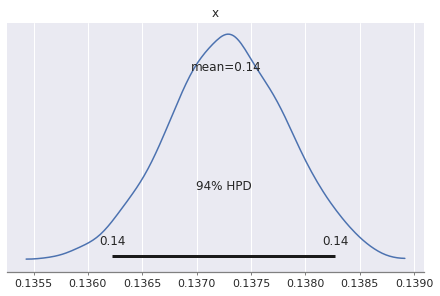

with model:
    distance_posterior = pm.sample_posterior_predictive(trace)

100%|██████████| 4000/4000 [00:04<00:00, 846.25it/s]

def calculate_prob_distance(angle, distance, ls):
    """
    Calculate the probability the ball will land inside the hole
    given the variance in angle and distance.
    
    NOTE: Adapted from Colin Carroll's Blog.
    """
    norm = scipy.stats.norm(0, 1)
    prob_angle = 2 * norm.cdf(
        np.arcsin((cup_radius - ball_radius) / ls) / angle) - 1
    prob_distance_one = norm.cdf(
        (DISTANCE_TOLERANCE - OVERSHOT) / ((ls + OVERSHOT) * distance)
    )
    prob_distance_two = norm.cdf(-OVERSHOT / ((ls + OVERSHOT) * distance))
    prob_distance = prob_distance_one - prob_distance_two
    
    return prob_angle * prob_distance

ls = np.linspace(0, new_df.distance.max(), 200)

new_df['success_prob'] = new_df.success_count / new_df.tries
sns.set()
plt.figure(figsize=(16, 6))
ax = sns.scatterplot(
    x='distance', 
    y='success_prob',
    data=new_df,
    label='Actual', 
    s=200
)
sns.scatterplot(
    x='distance', 
    y=new_geo_model_prob, 
    data=new_df, 
    label='Angle only Model',
    ax=ax, 
    color='red', 
    s=100
)

sns.scatterplot(
    x='distance', 
    y=calculate_prob_distance(
        trace['angle_of_shot_radians'].mean(), 
        trace['variance_of_distance'].mean(),
        new_df.distance
    ), 
    data=new_df, 
    label='Distance + Angle based Model ',
    ax=ax, 
    color='black', 
    s=100
)
ax.set(
    xlabel='Distance from hole(ft)', 
    ylabel='Probability of Success'
)

plt.setp(ax.get_legend().get_texts(), fontsize='25')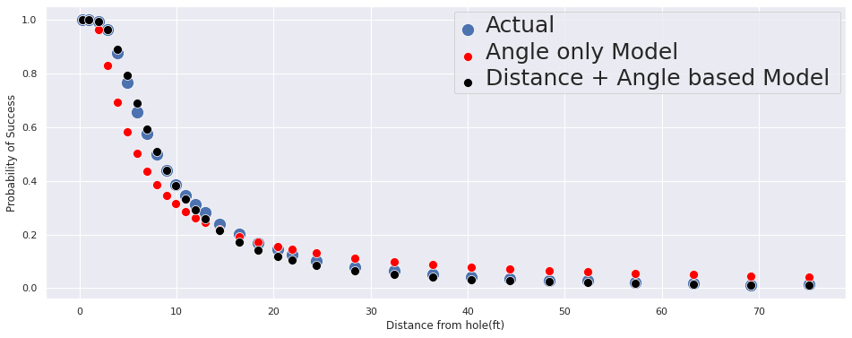

From the graph, we can conclude that:

• The model is good at distance lower than 10 ft and distances higher than 40ft.
• There is some mismatch between 10ft to 40ft, but overall this is a good fit.

What’s the point?

Using Bayesian analysis, we want to be able to quantify the unvertainity with each of our predictions. Since each prediction is a distribution, we can utilize this to see where the putts will fall if they do not fall in the hole.

def simulate_from_distance(trace, distance_to_hole, trials=10_000):
    n_samples = trace['angle_of_shot_radians'].shape[0]

    idxs = np.random.randint(0, n_samples, trials)
    variance_of_shot = trace['angle_of_shot_radians'][idxs]
    variance_of_distance = trace['variance_of_distance'][idxs]

    theta = np.random.normal(0, variance_of_shot)
    distance = np.random.normal(distance_to_hole + OVERSHOT, (distance_to_hole + OVERSHOT) * variance_of_distance)

    final_position = np.array([distance * np.cos(theta), distance * np.sin(theta)])

    made_it = np.abs(theta) < np.arcsin((cup_radius - ball_radius) / distance_to_hole)
    made_it = made_it * (final_position[0] > distance_to_hole) * (final_position[0] < distance_to_hole + DISTANCE_TOLERANCE)
    
    _, ax = plt.subplots()

    ax.plot(0, 0, 'k.', lw=1, mfc='black', ms=150 / distance_to_hole)
    ax.plot(*final_position[:, ~made_it], '.', alpha=0.1, mfc='r', ms=250 / distance_to_hole, mew=0.5)
    ax.plot(distance_to_hole, 0, 'ko', lw=1, mfc='black', ms=350 / distance_to_hole)

    ax.set_facecolor("#e6ffdb")
    ax.set_title(f"Final position of {trials:,d} putts from {distance_to_hole}ft.\n({100 * made_it.mean():.1f}% made)")
    return ax

simulate_from_distance(trace, distance_to_hole=10);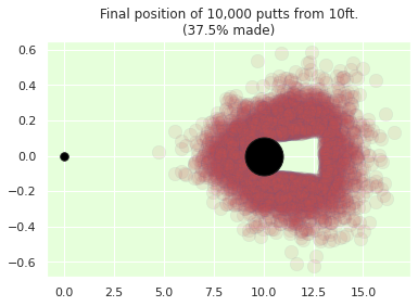

Conclusion

We’ve just seen how incorporate subjective knowledge in our models and help them fit cases that are specific to our use-case.

References:

• This is heavily inspired by Colin Caroll’s Blog present here
• The crux of this post is based on Dr. Gelman’s case study present here.