In our previous exploration, we analyzed 3,458 ConvFinQA records and established a curriculum learning framework with three difficulty stages: Easy (≤2 ops, simple context), Medium (2-3 ops, moderate complexity), and Hard (≥4 ops, complex multi-turn reasoning).

Now it’s time to put this curriculum to work by implementing and evaluating our models.

From Prompting to Programming

Traditionally, LLM applications rely on hand-rolled prompts—carefully crafted text instructions that are often brittle and difficult to optimize, especially for complex multi-step reasoning tasks like financial QA.

Our curriculum learning approach demands systematic experimentation across models, difficulty levels, and optimization strategies. This makes DSPy the ideal framework, as it transforms prompting from an art into systematic, testable code.

Why DSPy for curriculum learning?

Reproducible experiments: Prompts become Python objects → diffable, unit-testable, version-controlled
Optimization: Built-in optimizers (LabeledFewShot, BootstrapFewShot) auto-search the prompt space across our curriculum stages
Clean evaluation pipeline: First-class metrics support—plug in exact match, hit .compile(), get train/val loops with curriculum-aware sampling
Model flexibility: Test curriculum effects across GPT-4, o4-mini, Gemini, and open-source models with one-line swaps
Efficient iteration: Caching and threading speed up development cycles crucial for curriculum experiments

This approach lets us test whether our Easy→Medium→Hard curriculum improves financial reasoning compared to random sampling.

Evaluation Metrics

For this exploratory analysis, we need a clear metric to measure model performance across our curriculum learning experiments. Following the original ConvFinQA paper, we adopt Exact Match (EM) as our primary evaluation metric.

Primary Metric: Turn-level EM

Turn-level EM measures whether the generated answer for a specific dialogue turn exactly matches the gold standard answer. This binary metric (1 for exact match, 0 otherwise) provides a strict but interpretable measure of performance that directly aligns with the task requirements.

We choose this as our primary metric for several reasons: - Simplicity: Easy to implement and interpret for initial experimentation - Strictness: Financial reasoning requires precision—approximate answers can be misleading - Comparability: Direct comparison with baseline results from the original paper - Curriculum sensitivity: Clear signal for measuring improvement across difficulty levels

Additional Metrics (Future Work)

There are several other metrics could be useful:

Conversation-level metrics like Dialogue Mean EM and Joint EM would better capture multi-turn reasoning dependencies, but add complexity to curriculum design. Since our curriculum is based on individual example difficulty rather than conversation-level complexity, turn-level metrics are more appropriate for this phase.

Diagnostic metrics such as Exec-agree % and numeric error analysis would help distinguish between reasoning failures and execution errors. However, for establishing whether curriculum learning improves over random sampling, the binary success signal from exact match provides sufficient discriminative power.

Efficiency metrics like program length and evidence tokens could reveal interesting patterns about how curriculum learning affects model behavior, but are secondary to establishing basic performance improvements.

We’ve skipped the other metrics for now for the sake of brevity.

Model List

We will consider the following families of models:

Family	Rationale	Benchmarked Checkpoints
Non-Reasoning	Classic next-token predictors. Useful as baselines for curriculum-learning because they expose the value of explicit reasoning.	• `openai/gpt-4.1-2025-04-14` • `openai/gpt-4.1-mini-2025-04-14`
Reasoning	Architected for multi-step, chain-of-thought inference. Expected to excel once the curriculum introduces compositional tasks.	• `openai/o4-mini-2025-04-16` • `anthropic/claude-sonnet-4-20250514` • `gemini-2.5-flash` • `gemini-2.5-flash-lite`
Frontier	Flagship models from frontier labs. Highest quality but costly—kept only for upper-bound comparisons, not final deployment.	• `openai/o3-2025-04-16` • `anthropic/claude-opus-4-20250514` • `gemini-2.5-pro`
Open-Source	Critical for cost-sensitive deployments(an OS models FTW). Benchmarked to quantify the closed–open gap.	• `qwen3-32b`

Two-Stage Gating Protocol

Gate
• Dataset: 50 “Easy” teacher-forced dialogues
• Retain a model only if Turn-EM ≥ 0.55
Probe
• Dataset: 30 dialogues (15 Medium + 15 Hard), closed-loop
• Retain a model only if Final-Turn EM ≥ 0.35 and Dialogue-mean EM ≥ 0.35

This pipeline quickly eliminates weak candidates while preserving models whose strengths surface in longer, reasoning-heavy contexts.

Experiment Tracking

All training and evaluation runs are logged with MLflow:

MLflow Tracking – run metadata, metrics, and artifacts for DSPy experiments
MLflow Model – package DSPy programs for reproducible rollout
MLflow Evaluate – built-in GenAI evaluators for rapid iteration
MLflow Tracing – one-line capture of DSPy internals for debugging

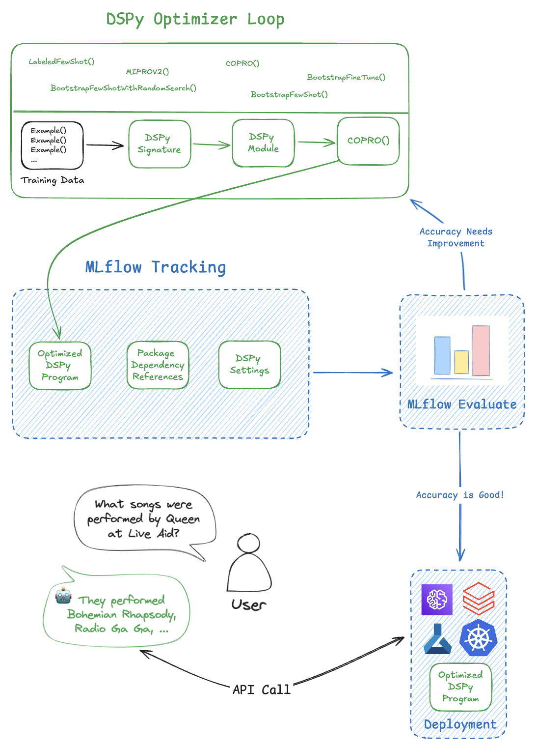
In production, the deployment pipeline would look as follows:

, ,
, _{, DSPy Production deployment with MLFlow. Source: MLFlow Docs,},

Setup

import mlflow
from IPython.display import IFrame, HTML, display

mlflow.set_tracking_uri("http://localhost:5000")
mlflow.dspy.autolog(log_compiles=True, log_evals=True, log_traces_from_compile=True)
result = mlflow.set_experiment("DSPy")

# Display MLFlow UI in an iframe to prevent HTML document conflicts
print(f"Experiment: {result.name} (ID: {result.experiment_id})")
display(HTML(f'<p><a href="http://localhost:5000/#/experiments/{result.experiment_id}" target="_blank">View MLFlow Experiment UI</a></p>'))

<Experiment: artifact_location='mlflow-artifacts:/1', creation_time=1753611058221, experiment_id='1', last_update_time=1753611058221, lifecycle_stage='active', name='DSPy', tags={}>

import os

import dotenv
import dspy

dotenv.load_dotenv("../.env")
MAX_TOKENS = 20_000

lm_oai_gpt_4_1 = dspy.LM(
    "openai/gpt-4.1-2025-04-14",
    api_key=os.environ["OPENAI_API_KEY"],
    max_tokens=MAX_TOKENS,
)
lm_oai_gpt_4_1_mini = dspy.LM(
    "openai/gpt-4.1-mini-2025-04-14",
    api_key=os.environ["OPENAI_API_KEY"],
    max_tokens=MAX_TOKENS,
)

lm_oai_o4_mini = dspy.LM(
    "openai/o4-mini-2025-04-16",
    api_key=os.environ["OPENAI_API_KEY"],
    temperature=1.0,
    max_tokens=MAX_TOKENS,
)
lm_anthropic_sonnet_4_0 = dspy.LM(
    "anthropic/claude-sonnet-4-20250514",
    api_key=os.environ["ANTHROPIC_API_KEY"],
    max_tokens=MAX_TOKENS,
)
lm_gemini_flash_2_5 = dspy.LM(
    "gemini/gemini-2.5-flash",
    api_key=os.environ["GEMINI_API_KEY"],
    max_tokens=MAX_TOKENS,
)
lm_gemini_flash_2_5_lite = dspy.LM(
    "gemini/gemini-2.5-flash-lite",
    api_key=os.environ["GEMINI_API_KEY"],
    max_tokens=MAX_TOKENS,
)

lm_oai_o3 = dspy.LM(
    "openai/o3-2025-04-16",
    api_key=os.environ["OPENAI_API_KEY"],
    temperature=1.0,
    max_tokens=MAX_TOKENS,
)
lm_anthropic_opus_4_0 = dspy.LM(
    "anthropic/claude-opus-4-20250514",
    api_key=os.environ["ANTHROPIC_API_KEY"],
    max_tokens=MAX_TOKENS,
)
lm_gemini_pro_2_5 = dspy.LM(
    "gemini/gemini-2.5-pro",
    api_key=os.environ["GEMINI_API_KEY"],
    max_tokens=MAX_TOKENS,
)

lm_qwen3_32b = dspy.LM(
    "ollama/qwen3:32b",
    api_base="http://localhost:11434",
    api_key="",
    max_tokens=MAX_TOKENS,
)

import dspy

llms = [
    lm_oai_gpt_4_1,
    lm_oai_gpt_4_1_mini,
    lm_oai_o4_mini,
    lm_anthropic_sonnet_4_0,
    lm_gemini_flash_2_5,
    lm_gemini_flash_2_5_lite,
    lm_oai_o3,
    lm_anthropic_opus_4_0,
    lm_gemini_pro_2_5,
    lm_qwen3_32b,
]


class Echo(dspy.Signature):
    """Echoes the input prompt."""

    prompt = dspy.InputField()
    output = dspy.OutputField()


with mlflow.start_run(run_name="Setup") as run:
    for lm in llms:
        try:
            with dspy.context(lm=lm, track_usage=True, cache=True):
                if lm in [lm_oai_gpt_4_1, lm_oai_gpt_4_1_mini]:
                    program = dspy.Predict("instruction -> answer")
                else:
                    program = dspy.ChainOfThought("instruction -> answer")
                response = program(instruction="What is the date?")
                if getattr(response, "reasoning", None):
                    print(f"{lm.model} Reasoning: {response.reasoning}")
                print(f"{lm.model}: {response.answer}")
        except Exception as e:
            print(f"{getattr(lm, 'model', lm)}: ERROR - {e}")

openai/gpt-4.1-2025-04-14: Today's date is June 13, 2024.
openai/gpt-4.1-mini-2025-04-14: The current date is June 15, 2024.
openai/o4-mini-2025-04-16 Reasoning: The user asked for the current date. I will provide today's date in a clear, human-readable format.
openai/o4-mini-2025-04-16: The current date is May 30, 2024.
anthropic/claude-sonnet-4-20250514 Reasoning: The user is asking for the current date. However, I don't have access to real-time information or the ability to know what the current date is. I should explain that I cannot provide the current date and suggest how they can find this information.
anthropic/claude-sonnet-4-20250514: I don't have access to real-time information, so I cannot tell you the current date. To find today's date, you can:
- Check your computer, phone, or other device
- Search "what is today's date" in a search engine
- Ask a voice assistant like Siri, Alexa, or Google Assistant
gemini/gemini-2.5-flash Reasoning: The user is asking for the current date. I will provide today's date.
gemini/gemini-2.5-flash: June 10, 2024
gemini/gemini-2.5-flash-lite Reasoning: The user is asking for the current date. I need to access the current date and format it as requested.
gemini/gemini-2.5-flash-lite: The current date is October 26, 2023.
openai/o3-2025-04-16 Reasoning: I don’t have real-time access to the system clock, so I’m unable to determine the exact current date at the moment of this response.
openai/o3-2025-04-16: I’m sorry, I don’t have access to real-time information to tell today’s date.
anthropic/claude-opus-4-20250514 Reasoning: The user is asking for the current date. However, as an AI assistant, I don't have access to real-time information and cannot provide the current date. I should explain this limitation clearly to the user.
anthropic/claude-opus-4-20250514: I don't have access to real-time information, so I cannot tell you today's date. To get the current date, you can check your device's calendar, search "what's today's date" in a search engine, or ask a voice assistant with real-time capabilities.
gemini/gemini-2.5-pro Reasoning: The user has asked for the current date. I will access my internal system's real-time clock to provide the current calendar date.
gemini/gemini-2.5-pro: Today's date is September 10, 2024.
ollama/qwen3:32b Reasoning: I cannot access real-time data or the current date. My knowledge is static and up to July 2024. To find the current date, please check your device's clock or calendar.
ollama/qwen3:32b: I cannot provide the current date as I do not have access to real-time information. Please check your device's clock or calendar for the current date.
🏃 View run Setup at: http://localhost:5000/#/experiments/1/runs/20df48ca1ad2461d9dcc0b1575caec6d
🧪 View experiment at: http://localhost:5000/#/experiments/1

import json

data = json.load(open("../data/convfinqa_dataset.json"))

Model Selection

In the easy problems stage, we will select a relatively straightforward implementation. Specifically, we will provide the model with all context, and ask it to answer the question in a zero-shot manner.

This will help us identify strong baseline performance, and identify any issues with the model’s ability to understand the problem.

First, we will create the DSPy signatures for our dataset. Signatures are used to define the input and output of a model.

Specifically, we will have two types of signatures: one that doesn’t support reasoning model(for direct prediction models like GPT-4.1), and one that does support reasoning mode(for the reasoning models like o3, gemini pro, etc.)

class SolveTurnWithoutReasoning(dspy.Signature):
    conversation_context: str = dspy.InputField(desc="Conversation so far")
    evidence_snippets: str = dspy.InputField(
        desc="Snippets of evidence surrounding the table"
    )
    table: str = dspy.InputField(desc="Input financial table with metrics")
    question: str = dspy.InputField(desc="Question to answer")

    ops: str = dspy.OutputField(
        desc="Comma-separated ConvFinQA DSL program. Allowed ops: add(x, y), subtract(x, y), multiply(x, y), divide(x, y), exp(x, y), greater(x, y). Args may be constants (e.g., const_100), numbers (int or float), or prior step refs (#0, #1…). Order always follows the pattern x <op> y—pick x and y deliberately. Example: subtract(const_100, 42), divide(#0, 3.14). Convert to percentages only if explicitly asked in the question."
    )
    answer: str = dspy.OutputField(
        desc="Final answer. This will be a single number, or a boolean string(yes/no)"
    )


class SolveTurnWithReasoning(dspy.Signature):
    conversation_context: str = dspy.InputField(desc="Conversation so far")
    evidence_snippets: str = dspy.InputField(
        desc="Snippets of evidence surrounding the table"
    )
    table: str = dspy.InputField(desc="Input financial table with metrics")
    question: str = dspy.InputField(desc="Question to answer")

    reasoning: str = dspy.OutputField(
        desc="Reasoning behind the answer. Carefully analyze the conversation_context, and especially the evidence_snippets and table for the given question, and generate your reasoning before generating the ops and answer."
    )
    ops: str = dspy.OutputField(
        desc="Comma-separated ConvFinQA DSL program. Allowed ops: add(x, y), subtract(x, y), multiply(x, y), divide(x, y), exp(x, y), greater(x, y). Args may be constants (e.g., const_100), numbers (int or float), or prior step refs (#0, #1…). Order always follows the pattern x <op> y—pick x and y deliberately. Example: subtract(const_100, 42), divide(#0, 3.14). Convert to percentages only if explicitly asked in the question."
    )
    answer: str = dspy.OutputField(
        desc="Final answer. This will be a single number, or a boolean string(yes/no)"
    )


class TurnSolver(dspy.Module):
    """
    In the context of this series of interconnected finance-related queries and the additional information provided by the pretext, table data, and posttext from a company's financial filings, please provide a response to the final question. This may require extracting information from the context and performing mathematical calculations. Please take into account the information provided in the preceding questions and their answers when formulating your response: \n\n
    """

    def __init__(self, reasoning_lm=False):
        super().__init__()
        if reasoning_lm:
            self.pred = dspy.ChainOfThought(SolveTurnWithReasoning)
        else:
            self.pred = dspy.Predict(SolveTurnWithoutReasoning)

    def forward(self, conversation_context, evidence_snippets, table, question):
        """
        Run the model to solve a single turn.

        Args:
            conversation_context (str): Conversation so far.
            evidence_snippets (str): Evidence text around the table.
            table (str): Financial table in markdown.
            question (str): Question to answer.

        Returns:
            dspy.Prediction: Model output with reasoning, ops, and answer.
        """
        return self.pred(
            conversation_context=conversation_context,
            evidence_snippets=evidence_snippets,
            table=table,
            question=question,
        )

Next, we define a few helper functions to format our dataset for the DSPy model. We intentionally don’t spend too much time here for now, and will come back to this later, during the optimization phase.

def norm_ans(x):
    """
    Normalize an answer for comparison.

    Converts input to string, strips whitespace, removes percent signs,
    and attempts to cast to float. If conversion fails, returns the cleaned string.

    Args:
        x: The answer to normalize (str, float, or int).

    Returns:
        float or str: Normalized float if possible, else cleaned string.
    """
    s = str(x).strip().replace("%", "")
    try:
        return float(s)
    except Exception:
        return s


def _table_md(table_dict: dict, max_cols: int | None = None) -> str:
    """
    Convert a dictionarised table to compact GitHub-markdown.

    Accepted shapes
    1) {row_name: {col_name: value, …}, …}   # regular 2-level mapping
    2) {col_name: value, …}                  # flat → coerced to single row

    Guarantees
    • Original row order is kept.
    • Column headers are kept in *first-seen* order; NO deduplication.
    • max_cols (if given) truncates *after* enumeration, duplicates included.
    • None → "" and everything else is str()-ed.
    """
    if not table_dict:
        return ""

    if all(not isinstance(v, dict) for v in table_dict.values()):
        # flat mapping → one anonymous row
        table_dict = {"": dict(table_dict)}
    else:
        # ensure every value is a dict
        table_dict = {
            r: (v if isinstance(v, dict) else {"": v}) for r, v in table_dict.items()
        }

    row_ids = list(table_dict.keys())  # preserve caller order

    cols: list = []
    for r in row_ids:
        cols.extend(table_dict[r].keys())
    if max_cols is not None:
        cols = cols[:max_cols]

    header = "| Row | " + " | ".join(map(str, cols)) + " |"
    sep = "|" + "---|" * (len(cols) + 1)
    lines = [header, sep]

    for r in row_ids:
        vals = [str(table_dict[r].get(c, "")) for c in cols]
        lines.append("| " + str(r) + " | " + " | ".join(vals) + " |")

    return "\n".join(lines)


def build_inputs_from_row(
    row,
    turn_idx,
    *,
    history_mode: str = "teacher",
    state: dict | None = None,
    max_table_cols: int = 100,
):
    """
    history_mode: 'teacher' | 'model' | 'none'
    state: carries model predictions across turns when history_mode='model'
           expected keys: {'pred_answers': list[str|float]}
    evidence_builder: optional callable(row, turn_idx)->str; if None, use simple truncation.
    """
    qs = row["dialogue_conv_questions"]
    gold = row["dialogue_executed_answers"]

    # ---- history ----
    history_lines = []
    for t in range(turn_idx):
        history_lines.append(f"Q{t + 1}: {qs[t]}")
        if history_mode == "teacher":
            history_lines.append(f"A{t + 1}: {gold[t]}")
        elif (
            history_mode == "model" and state and len(state.get("pred_answers", [])) > t
        ):
            history_lines.append(f"A{t + 1}: {state['pred_answers'][t]}")
        elif history_mode == "none":
            pass  # only questions
    conversation_context = "\n".join(history_lines) if history_lines else "None"

    # compact pre/post: first N sentences
    # def first_sents(txt, n):
    #     if not txt: return ""
    #     # very light sentence split
    #     parts = [p.strip() for p in txt.split(". ") if p.strip()]
    #     return ". ".join(parts[:n])
    # pre = first_sents(row.get("doc_pre_text", "") or "", max_pre_sents)
    # post= first_sents(row.get("doc_post_text", "") or "", max_post_sents)
    # evidence_snippets = f"[PRE]\n{pre}\n[/PRE]\n[POST]\n{post}\n[/POST]"
    evidence_snippets = (
        f"[PRE]\n{row['doc_pre_text']}\n[/PRE]\n[POST]\n{row['doc_post_text']}\n[/POST]"
    )
    table_md = _table_md(row.get("doc_table", {}) or {}, max_cols=max_table_cols)

    return dict(
        conversation_context=conversation_context,
        evidence_snippets=evidence_snippets,
        table=table_md,
        question=qs[turn_idx],
        **row,
    )

def evaluate_dialogues(model, df):
    """
    Evaluate a dialogue model on a DataFrame of conversations.

    Args:
        model: Callable that takes unpacked input dict and returns an object with at least `.answer` (and optionally `.ops`).
        df: pd.DataFrame with columns:
            - "dialogue_conv_questions": list of str, all questions in the conversation
            - "dialogue_executed_answers": list of str/float, all executed answers so far
            - (other columns as needed by evidence_builder)

    Returns:
        dict with:
            - "turn_em_micro": float, micro-averaged exact match over all turns
            - "dlg_mean_em_macro": float, macro-averaged mean EM per dialogue
            - "joint_em": float, fraction of dialogues with all turns correct
            - "final_turn_em": float, EM on the final turn of each dialogue
            - "n_dialogues": int, number of dialogues
            - "n_turns": int, total number of turns
    """
    turn_hits = 0
    turn_tot = 0
    # exec_hits = 0
    dlg_mean_ems = []
    dlg_joint_hits = 0
    final_hits = 0

    for _, row in df.iterrows():
        qs = row["dialogue_conv_questions"]
        gold = row["dialogue_executed_answers"]
        ems = []
        exec_flags = []
        for t in range(len(qs)):
            inp = build_inputs_from_row(row, t)
            out = model(**inp)  # out.ops, out.answer
            pa = norm_ans(out.answer)
            ga = norm_ans(gold[t])
            em = float(pa == ga)
            ems.append(em)
            turn_hits += em
            turn_tot += 1

            # (optional) exec check if you have your python DSL evaluator:
            # exec_ok = False
            # try:
            #     # exec_ok = (run_dsl(out.ops, inp) == ga)   # plug your interpreter
            #     exec_ok = False
            # except Exception:
            #     exec_ok = False
            # exec_flags.append(exec_ok)
            # exec_hits += float(exec_ok)

        dlg_mean_ems.append(sum(ems) / len(ems))
        if all(v == 1.0 for v in ems):
            dlg_joint_hits += 1
        final_hits += ems[-1]

    return {
        "turn_em_micro": turn_hits / max(1, turn_tot),
        "dlg_mean_em_macro": sum(dlg_mean_ems) / max(1, len(dlg_mean_ems)),
        "joint_em": dlg_joint_hits / max(1, len(dlg_mean_ems)),
        "final_turn_em": final_hits / max(1, len(dlg_mean_ems)),
        # "exec_agree_rate": exec_hits / max(1, turn_tot),
        "n_dialogues": len(dlg_mean_ems),
        "n_turns": turn_tot,
    }

Next, we will create the DSPy metric, used to evaluate the performance of our model.

We will focus on 2 parts to our metric: - If the answer is a floating point number, we will aim to compare it with the ground truth with some tolerance. - If the answer is a string, we will aim to perform exact match via DSPy’s exact_match metric.

def turn_em_metric(example, pred, trace=None):
    """
    Compute turn-level exact match (EM) metric for a single example/prediction pair.

    Args:
        example: dict-like, must contain "gold_answer" key.
        pred: object with an "answer" attribute.

    Returns:
        float: 1.0 if normalized prediction matches normalized gold answer (with tolerance for floats), else 0.0.
    """
    from dspy.evaluate.metrics import answer_exact_match

    pa = norm_ans(pred.answer)
    ga = norm_ans(example["answer"])
    if isinstance(pa, float) and isinstance(ga, float):
        return float(abs(pa - ga) <= 1e-2)
    else:
        # exact_match in DSPy needs the inputs to be in string format
        # due to the normalisations DSPy performs internally.
        ground_truth = dspy.Prediction(answer=str(example.answer))
        pred_answer = dspy.Prediction(answer=str(pred.answer))
        return float(answer_exact_match(ground_truth, pred_answer))

def to_turn_examples(df, history_mode="teacher"):
    examples = []
    for _, row in df.iterrows():
        qs = row["dialogue_conv_questions"]
        gold = row["dialogue_executed_answers"]
        for t in range(len(qs)):
            inp = build_inputs_from_row(row, t, history_mode=history_mode)
            ex = dict(**inp, answer=gold[t])
            examples.append(
                dspy.Example(**ex).with_inputs(
                    "conversation_context",
                    "evidence_snippets",
                    "table",
                    "question",
                )
            )
    return examples

Next, we will prepare our datasets.

We will aim to use the splits as follows: - train: Used primarily for the optimisation phase. This will be discussed shortly. - valid: Used to evaluate the performance of an LM on an optimised model trained using the train dataset. - test: Used to evaluate the performance of an LM on a held-out dataset. This will determine the overall stage performance.

import pandas as pd

train_df = pd.DataFrame(data["train"])
test_df = pd.DataFrame(data["dev"])

# Flatten features to remove the indexing gymnastics
train_flat_df = pd.concat(
    [
        train_df.drop(["doc", "dialogue", "features"], axis=1),
        train_df["doc"].apply(pd.Series).add_prefix("doc_"),
        train_df["dialogue"].apply(pd.Series).add_prefix("dialogue_"),
        train_df["features"].apply(pd.Series).add_prefix("features_"),
    ],
    axis=1,
)

test_flat_df = pd.concat(
    [
        test_df.drop(["doc", "dialogue", "features"], axis=1),
        test_df["doc"].apply(pd.Series).add_prefix("doc_"),
        test_df["dialogue"].apply(pd.Series).add_prefix("dialogue_"),
        test_df["features"].apply(pd.Series).add_prefix("features_"),
    ],
    axis=1,
)

train_flat_df.head()

	id	doc_pre_text	doc_post_text	doc_table	dialogue_conv_questions	dialogue_conv_answers	dialogue_turn_program	dialogue_executed_answers	dialogue_qa_split	features_num_dialogue_turns	features_has_type2_question	features_has_duplicate_columns	features_has_non_numeric_values
0	Single_JKHY/2009/page_28.pdf-3	26 \| 2009 annual report in fiscal 2008 , revenues in the credit un...	year ended june 30 , cash provided by operations increased $ 25587...	{'Year ended June 30, 2009': {'net income': 103102.0, 'non-cash ex...	[what is the net cash from operating activities in 2009?, what abo...	[206588, 181001, 25587, 14.1%]	[206588, 181001, subtract(206588, 181001), subtract(206588, 181001...	[206588.0, 181001.0, 25587.0, 0.14136]	[False, False, False, False]	4	False	False	False
1	Single_RSG/2008/page_114.pdf-2	substantially all of the goodwill and other intangible assets reco...	the above unaudited pro forma financial information includes adjus...	{'year ended december 31 2008 ( unaudited )': {'revenue': 9362.2, ...	[what were revenues in 2008?, what were they in 2007?, what was th...	[9362.2, 9244.9, 117.3, 1.3%]	[9362.2, 9244.9, subtract(9362.2, 9244.9), subtract(9362.2, 9244.9...	[9362.2, 9244.9, 117.3, 0.01269]	[False, False, False, False]	4	False	False	False
2	Single_AAPL/2002/page_23.pdf-1	in a new business model such as the retail segment is inherently r...	.	{'2002': {'net sales': 5742.0, 'cost of sales': 4139.0, 'gross mar...	[what was the total of net sales in 2001?, and what was that in 20...	[5363, 7983, -2620, -32%]	[5363, 7983, subtract(5363, 7983), subtract(5363, 7983), divide(#0...	[5363.0, 7983.0, -2620.0, -0.3282]	[False, False, False, False]	4	False	False	False
3	Single_UPS/2009/page_33.pdf-2	( 1 ) includes shares repurchased through our publicly announced s...	.	{'12/31/04': {'united parcel service inc .': 100.0, 's&p 500 index...	[what was the change in the performance of the united parcel servi...	[-24.05, -24.05%, 102.11, 2.11, 2.11%, -26.16%]	[subtract(75.95, const_100), subtract(75.95, const_100), divide(#0...	[-24.05, -0.2405, 102.11, 2.11, 0.0211, -0.2616]	[False, False, False, False, False, False]	6	False	False	False
4	Double_UPS/2009/page_33.pdf	( 1 ) includes shares repurchased through our publicly announced s...	.	{'12/31/04': {'united parcel service inc .': 100.0, 's&p 500 index...	[what was the fluctuation of the performance price of the ups from...	[-8.94, -8.9%, -24.05, -24.05%, 2.11, 2.11%, -26.16%]	[subtract(91.06, const_100), subtract(91.06, const_100), divide(#0...	[-8.94, -0.0894, -24.05, -0.2405, 2.11, 0.0211, -0.2616]	[False, False, True, True, True, True, True]	7	True	False	False

easy_train_ids = pd.read_json("./splits/easy_train.jsonl", lines=True)
easy_valid_ids = pd.read_json("./splits/easy_valid.jsonl", lines=True)
easy_test_ids = pd.read_json("./splits/easy_test.jsonl", lines=True)

medium_train_ids = pd.read_json("./splits/medium_train.jsonl", lines=True)
medium_valid_ids = pd.read_json("./splits/medium_valid.jsonl", lines=True)
medium_test_ids = pd.read_json("./splits/medium_test.jsonl", lines=True)

hard_train_ids = pd.read_json("./splits/hard_train.jsonl", lines=True)
hard_valid_ids = pd.read_json("./splits/hard_valid.jsonl", lines=True)
hard_test_ids = pd.read_json("./splits/hard_test.jsonl", lines=True)

easy_train_df = train_flat_df[train_flat_df["id"].isin(easy_train_ids["id"])].copy()
easy_valid_df = train_flat_df[train_flat_df["id"].isin(easy_valid_ids["id"])].copy()
easy_test_df = test_flat_df[test_flat_df["id"].isin(easy_test_ids["id"])].copy()

medium_train_df = train_flat_df[train_flat_df["id"].isin(medium_train_ids["id"])].copy()
medium_valid_df = train_flat_df[train_flat_df["id"].isin(medium_valid_ids["id"])].copy()
medium_test_df = test_flat_df[test_flat_df["id"].isin(medium_test_ids["id"])].copy()

hard_train_df = train_flat_df[train_flat_df["id"].isin(hard_train_ids["id"])].copy()
hard_valid_df = train_flat_df[train_flat_df["id"].isin(hard_valid_ids["id"])].copy()
hard_test_df = test_flat_df[test_flat_df["id"].isin(hard_test_ids["id"])].copy()

assert easy_train_ids.shape[0] == easy_train_df.shape[0]
assert easy_valid_ids.shape[0] == easy_valid_df.shape[0]
assert easy_test_ids.shape[0] == easy_test_df.shape[0]
assert medium_train_ids.shape[0] == medium_train_df.shape[0]
assert medium_valid_ids.shape[0] == medium_valid_df.shape[0]
assert medium_test_ids.shape[0] == medium_test_df.shape[0]
assert hard_train_ids.shape[0] == hard_train_df.shape[0]
assert hard_valid_ids.shape[0] == hard_valid_df.shape[0]
assert hard_test_ids.shape[0] == hard_test_df.shape[0]

easy_train_examples = to_turn_examples(easy_train_df)
easy_valid_examples = to_turn_examples(easy_valid_df)
easy_test_examples = to_turn_examples(easy_test_df)

len(easy_train_examples + easy_valid_examples)

We will used DSPy’s Evaluate class to run our evals in parallel(internally, this is just implemented via threads)

To ensure our setup works as expected, we will run a simple test first.

from dspy.evaluate import Evaluate

evaluator = Evaluate(
    devset=easy_valid_examples[:10],
    num_threads=32,
    display_progress=True,
    display_table=True,
    provide_traceback=True,
    return_all_scores=True,
    return_outputs=True,
)


from copy import deepcopy

tlm = deepcopy(lm_oai_gpt_4_1)
tlm.cache = False

# HACK: Weird bug in dspy where the context doesn't set the cache to False, causing answers to be returned from memory. I've found that creating a deepcopy and setting the attribute manually fixes this.
with dspy.context(lm=tlm) as ctx:
    evaluator(TurnSolver(reasoning_lm=False), metric=turn_em_metric)

Average Metric: 8.00 / 10 (80.0%): 100%|██████████| 10/10 [00:02<00:00,  3.48it/s]
🏃 View run eval at: http://localhost:5000/#/experiments/1/runs/a5433773d6ef4e359825412ad138c520
🧪 View experiment at: http://localhost:5000/#/experiments/1

2025/07/28 18:18:42 INFO dspy.evaluate.evaluate: Average Metric: 8.0 / 10 (80.0%)

	conversation_context	evidence_snippets	table	question	id	doc_pre_text	doc_post_text	doc_table	dialogue_conv_questions	dialogue_conv_answers	...	dialogue_executed_answers	dialogue_qa_split	features_num_dialogue_turns	features_has_type2_question	features_has_duplicate_columns	features_has_non_numeric_values	example_answer	ops	pred_answer	turn_em_metric
0	None	[PRE] entergy corporation and subsidiaries management's financial ...	\| Row \| 2009 net revenue \| volume/weather \| retail electric price ...	what was the difference in net revenue between 2009 and 2010?	Single_ETR/2011/page_22.pdf-3	entergy corporation and subsidiaries management's financial discus...	the volume/weather variance is primarily due to an increase of 836...	{'amount ( in millions )': {'2009 net revenue': 4694.0, 'volume/we...	['what was the difference in net revenue between 2009 and 2010?', ...	[357, 4694, 7.61%]	...	[357.0, 4694.0, 0.07605]	[False, False, False]	3	False	False	False	357.00000	subtract(2010 net revenue, 2009 net revenue)	357.0	✔️ [1.000]
1	Q1: what was the difference in net revenue between 2009 and 2010?\...	[PRE] entergy corporation and subsidiaries management's financial ...	\| Row \| 2009 net revenue \| volume/weather \| retail electric price ...	and the specific value for 2009 again?	Single_ETR/2011/page_22.pdf-3	entergy corporation and subsidiaries management's financial discus...	the volume/weather variance is primarily due to an increase of 836...	{'amount ( in millions )': {'2009 net revenue': 4694.0, 'volume/we...	['what was the difference in net revenue between 2009 and 2010?', ...	[357, 4694, 7.61%]	...	[357.0, 4694.0, 0.07605]	[False, False, False]	3	False	False	False	4694.00000	4694.0	4694.0	✔️ [1.000]
2	Q1: what was the difference in net revenue between 2009 and 2010?\...	[PRE] entergy corporation and subsidiaries management's financial ...	\| Row \| 2009 net revenue \| volume/weather \| retail electric price ...	so what was the percentage change during this time?	Single_ETR/2011/page_22.pdf-3	entergy corporation and subsidiaries management's financial discus...	the volume/weather variance is primarily due to an increase of 836...	{'amount ( in millions )': {'2009 net revenue': 4694.0, 'volume/we...	['what was the difference in net revenue between 2009 and 2010?', ...	[357, 4694, 7.61%]	...	[357.0, 4694.0, 0.07605]	[False, False, False]	3	False	False	False	0.07605	subtract(5051.0, 4694.0), divide(#0, 4694.0), multiply(#1, const_100)	7.61
3	None	[PRE] entergy new orleans , inc . management's financial discussio...	\| Row \| 2003 net revenue \| base rates \| volume/weather \| 2004 defe...	what was the net revenue in 2004?	Single_ETR/2004/page_258.pdf-4	entergy new orleans , inc . management's financial discussion and ...	the increase in base rates was effective june 2003 . the rate incr...	{'( in millions )': {'2003 net revenue': 208.3, 'base rates': 10.6...	[what was the net revenue in 2004?, what was the net revenue in 20...	[239.0, 208.3, 30.7, 14.7%]	...	[239.0, 208.3, 30.7, 0.14738]	[False, False, False, False]	4	False	False	False	239.00000	None	239.0	✔️ [1.000]
4	Q1: what was the net revenue in 2004?\nA1: 239.0	[PRE] entergy new orleans , inc . management's financial discussio...	\| Row \| 2003 net revenue \| base rates \| volume/weather \| 2004 defe...	what was the net revenue in 2003?	Single_ETR/2004/page_258.pdf-4	entergy new orleans , inc . management's financial discussion and ...	the increase in base rates was effective june 2003 . the rate incr...	{'( in millions )': {'2003 net revenue': 208.3, 'base rates': 10.6...	[what was the net revenue in 2004?, what was the net revenue in 20...	[239.0, 208.3, 30.7, 14.7%]	...	[239.0, 208.3, 30.7, 0.14738]	[False, False, False, False]	4	False	False	False	208.30000	None	208.3	✔️ [1.000]
5	Q1: what was the net revenue in 2004?\nA1: 239.0\nQ2: what was the...	[PRE] entergy new orleans , inc . management's financial discussio...	\| Row \| 2003 net revenue \| base rates \| volume/weather \| 2004 defe...	what was the change in value?	Single_ETR/2004/page_258.pdf-4	entergy new orleans , inc . management's financial discussion and ...	the increase in base rates was effective june 2003 . the rate incr...	{'( in millions )': {'2003 net revenue': 208.3, 'base rates': 10.6...	[what was the net revenue in 2004?, what was the net revenue in 20...	[239.0, 208.3, 30.7, 14.7%]	...	[239.0, 208.3, 30.7, 0.14738]	[False, False, False, False]	4	False	False	False	30.70000	subtract(239.0, 208.3)	30.7	✔️ [1.000]
6	Q1: what was the net revenue in 2004? A1: 239.0 Q2: what was the n...	[PRE] entergy new orleans , inc . management's financial discussio...	\| Row \| 2003 net revenue \| base rates \| volume/weather \| 2004 defe...	what is the percent change?	Single_ETR/2004/page_258.pdf-4	entergy new orleans , inc . management's financial discussion and ...	the increase in base rates was effective june 2003 . the rate incr...	{'( in millions )': {'2003 net revenue': 208.3, 'base rates': 10.6...	[what was the net revenue in 2004?, what was the net revenue in 20...	[239.0, 208.3, 30.7, 14.7%]	...	[239.0, 208.3, 30.7, 0.14738]	[False, False, False, False]	4	False	False	False	0.14738	subtract(239.0, 208.3), divide(#0, 208.3), multiply(#1, 100)	14.72
7	None	[PRE] nike , inc . notes to consolidated financial statements 2014...	\| Row \| severance and related costs \| cash payments \| non-cash sto...	what was the value of the sale of the starter brand?	Single_NKE/2009/page_81.pdf-1	nike , inc . notes to consolidated financial statements 2014 ( con...	the accrual balance as of may 31 , 2009 will be relieved throughou...	{'$ 2014': {'severance and related costs': 195.0, 'cash payments':...	['what was the value of the sale of the starter brand?', 'what was...	[60.0, 28.6, 31.4, 91%]	...	[60.0, 28.6, 31.4, 0.91083]	[False, False, False, False]	4	False	False	False	60.00000	None	60.0	✔️ [1.000]
8	Q1: what was the value of the sale of the starter brand?\nA1: 60.0	[PRE] nike , inc . notes to consolidated financial statements 2014...	\| Row \| severance and related costs \| cash payments \| non-cash sto...	what was the gain resulting from the sale?	Single_NKE/2009/page_81.pdf-1	nike , inc . notes to consolidated financial statements 2014 ( con...	the accrual balance as of may 31 , 2009 will be relieved throughou...	{'$ 2014': {'severance and related costs': 195.0, 'cash payments':...	['what was the value of the sale of the starter brand?', 'what was...	[60.0, 28.6, 31.4, 91%]	...	[60.0, 28.6, 31.4, 0.91083]	[False, False, False, False]	4	False	False	False	28.60000	None	28.6	✔️ [1.000]
9	Q1: what was the value of the sale of the starter brand?\nA1: 60.0...	[PRE] nike , inc . notes to consolidated financial statements 2014...	\| Row \| severance and related costs \| cash payments \| non-cash sto...	what was the change in value?	Single_NKE/2009/page_81.pdf-1	nike , inc . notes to consolidated financial statements 2014 ( con...	the accrual balance as of may 31 , 2009 will be relieved throughou...	{'$ 2014': {'severance and related costs': 195.0, 'cash payments':...	['what was the value of the sale of the starter brand?', 'what was...	[60.0, 28.6, 31.4, 91%]	...	[60.0, 28.6, 31.4, 0.91083]	[False, False, False, False]	4	False	False	False	31.40000	subtract(60.0, 28.6)	31.4	✔️ [1.000]

10 rows × 21 columns

import random

random.seed(42)

bootstrap_rs_random_easy_subset = random.sample(easy_train_examples, 70)

import re

import litellm
from dspy.teleprompt import BootstrapFewShotWithRandomSearch

# Config needed to prevent the optimizer from using _unsupported_ temperature
# for reasoning models.
litellm.drop_params = True


config = dict(
    max_bootstrapped_demos=3,
    max_labeled_demos=2,
    num_candidate_programs=5,
    num_threads=32,
    max_rounds=1,
)

bootstrap_rs_easy_compiled_programs = []

with mlflow.start_run(run_name="bootstrap_few_shot_rs_easy"):
    for candidate_lm in selected_llms:
        run_name = f"bootstrap_few_shot_rs_{candidate_lm.model.replace('/', '_')}"
        sanitized_run_name = re.sub(r"[^a-zA-Z0-9_\-]", "_", run_name)
        with mlflow.start_run(run_name=sanitized_run_name, nested=True):
            with dspy.context(lm=candidate_lm) as ctx:
                teleprompter = BootstrapFewShotWithRandomSearch(
                    metric=turn_em_metric, **config
                )
                optimized_program = teleprompter.compile(
                    dspy.ChainOfThought(SolveTurnWithReasoning),
                    trainset=bootstrap_rs_random_easy_subset,
                )
                bootstrap_rs_easy_compiled_programs.append(optimized_program)

Going to sample between 1 and 3 traces per predictor.
Will attempt to bootstrap 5 candidate sets.
Average Metric: 45.00 / 70 (64.3%): 100%|██████████| 70/70 [00:00<00:00, 87.74it/s] 
...
2025/07/29 01:09:48 INFO dspy.evaluate.evaluate: Average Metric: 56.0 / 70 (80.0%)

From the above, it looks like GPT-4.1 gives an score of 80% on the validation set, WITHOUT ANY PROMPT ENGINEERING/FEW-SHOT PROMPTING. This is great!

As mentioned earlier, due to cost and time constraints, we want to first narrow down the list of models we want to test on the harder stages.

As a recap, our implementation strategy here will be as follows: instead of just using the performance of the models on the “easy” validation set, we will use a combination of two datasets:

Gate - 50 Easy dialogs, teacher - forced. Drop model if Turn-EM < 0.55.
Probe - 30-dialog mixed micro-set (15 Medium + 15 Hard, closed loop). Keep model only if Final-Turn EM ≥ 0.35, Dialogue-mean EM ≥ 0.35

We will now create our “gate” and “probe” datasets.

gate_ids = easy_valid_ids.sample(50, random_state=42)
probe_medium_ids = medium_valid_ids.sample(15, random_state=42)
probe_hard_ids = hard_valid_ids.sample(30, random_state=42)

gate_df = easy_valid_df[easy_valid_df["id"].isin(gate_ids["id"])].copy()
probe_df = pd.concat(
    [
        medium_valid_df[medium_valid_df["id"].isin(probe_medium_ids["id"])],
        hard_valid_df[hard_valid_df["id"].isin(probe_hard_ids["id"])],
    ]
).copy()

assert gate_df.shape[0] == gate_ids.shape[0]
assert probe_df.shape[0] == probe_medium_ids.shape[0] + probe_hard_ids.shape[0]

gate_examples = to_turn_examples(gate_df, history_mode="teacher")
probe_examples = to_turn_examples(probe_df, history_mode="teacher")

We will also save the gate and probe dataset ids, to compare performance of different models on them.

import os

os.makedirs("validation_datasets", exist_ok=True)

gate_ids.to_json("validation_datasets/gate_ids.jsonl", orient="records", lines=True)
probe_medium_ids.to_json(
    "validation_datasets/probe_medium_ids.jsonl", orient="records", lines=True
)
probe_hard_ids.to_json(
    "validation_datasets/probe_hard_ids.jsonl", orient="records", lines=True
)

gate_examples[0].toDict()

{'conversation_context': 'None',
 'evidence_snippets': "[PRE]\nentergy corporation and subsidiaries management's financial discussion and analysis refer to 201cselected financial data - five-year comparison of entergy corporation and subsidiaries 201d which accompanies entergy corporation 2019s financial statements in this report for further information with respect to operating statistics . in november 2007 the board approved a plan to pursue a separation of entergy 2019s non-utility nuclear business from entergy through a spin-off of the business to entergy shareholders . in april 2010 , entergy announced that it planned to unwind the business infrastructure associated with the proposed spin-off transaction . as a result of the plan to unwind the business infrastructure , entergy recorded expenses in 2010 for the write-off of certain capitalized costs incurred in connection with the planned spin-off transaction . these costs are discussed in more detail below and throughout this section . net revenue utility following is an analysis of the change in net revenue comparing 2010 to 2009 . amount ( in millions ) .\n[/PRE]\n[POST]\nthe volume/weather variance is primarily due to an increase of 8362 gwh , or 8% ( 8 % ) , in billed electricity usage in all retail sectors , including the effect on the residential sector of colder weather in the first quarter 2010 compared to 2009 and warmer weather in the second and third quarters 2010 compared to 2009 . the industrial sector reflected strong sales growth on continuing signs of economic recovery . the improvement in this sector was primarily driven by inventory restocking and strong exports with the chemicals , refining , and miscellaneous manufacturing sectors leading the improvement . the retail electric price variance is primarily due to : increases in the formula rate plan riders at entergy gulf states louisiana effective november 2009 , january 2010 , and september 2010 , at entergy louisiana effective november 2009 , and at entergy mississippi effective july 2009 ; a base rate increase at entergy arkansas effective july 2010 ; rate actions at entergy texas , including base rate increases effective in may and august 2010 ; a formula rate plan provision of $ 16.6 million recorded in the third quarter 2009 for refunds that were made to customers in accordance with settlements approved by the lpsc ; and the recovery in 2009 by entergy arkansas of 2008 extraordinary storm costs , as approved by the apsc , which ceased in january 2010 . the recovery of storm costs is offset in other operation and maintenance expenses . see note 2 to the financial statements for further discussion of the proceedings referred to above. .\n[/POST]",
 'table': '| Row | 2009 net revenue | volume/weather | retail electric price | provision for regulatory proceedings | rough production cost equalization | ano decommissioning trust | fuel recovery | other | 2010 net revenue |\n|---|---|---|---|---|---|---|---|---|---|\n| amount ( in millions ) | 4694.0 | 231.0 | 137.0 | 26.0 | 19.0 | -24.0 | -44.0 | 12.0 | 5051.0 |',
 'question': 'what was the difference in net revenue between 2009 and 2010?',
 'id': 'Single_ETR/2011/page_22.pdf-3',
 'doc_pre_text': "entergy corporation and subsidiaries management's financial discussion and analysis refer to 201cselected financial data - five-year comparison of entergy corporation and subsidiaries 201d which accompanies entergy corporation 2019s financial statements in this report for further information with respect to operating statistics . in november 2007 the board approved a plan to pursue a separation of entergy 2019s non-utility nuclear business from entergy through a spin-off of the business to entergy shareholders . in april 2010 , entergy announced that it planned to unwind the business infrastructure associated with the proposed spin-off transaction . as a result of the plan to unwind the business infrastructure , entergy recorded expenses in 2010 for the write-off of certain capitalized costs incurred in connection with the planned spin-off transaction . these costs are discussed in more detail below and throughout this section . net revenue utility following is an analysis of the change in net revenue comparing 2010 to 2009 . amount ( in millions ) .",
 'doc_post_text': 'the volume/weather variance is primarily due to an increase of 8362 gwh , or 8% ( 8 % ) , in billed electricity usage in all retail sectors , including the effect on the residential sector of colder weather in the first quarter 2010 compared to 2009 and warmer weather in the second and third quarters 2010 compared to 2009 . the industrial sector reflected strong sales growth on continuing signs of economic recovery . the improvement in this sector was primarily driven by inventory restocking and strong exports with the chemicals , refining , and miscellaneous manufacturing sectors leading the improvement . the retail electric price variance is primarily due to : increases in the formula rate plan riders at entergy gulf states louisiana effective november 2009 , january 2010 , and september 2010 , at entergy louisiana effective november 2009 , and at entergy mississippi effective july 2009 ; a base rate increase at entergy arkansas effective july 2010 ; rate actions at entergy texas , including base rate increases effective in may and august 2010 ; a formula rate plan provision of $ 16.6 million recorded in the third quarter 2009 for refunds that were made to customers in accordance with settlements approved by the lpsc ; and the recovery in 2009 by entergy arkansas of 2008 extraordinary storm costs , as approved by the apsc , which ceased in january 2010 . the recovery of storm costs is offset in other operation and maintenance expenses . see note 2 to the financial statements for further discussion of the proceedings referred to above. .',
 'doc_table': {'amount ( in millions )': {'2009 net revenue': 4694.0,
   'volume/weather': 231.0,
   'retail electric price': 137.0,
   'provision for regulatory proceedings': 26.0,
   'rough production cost equalization': 19.0,
   'ano decommissioning trust': -24.0,
   'fuel recovery': -44.0,
   'other': 12.0,
   '2010 net revenue': 5051.0}},
 'dialogue_conv_questions': ['what was the difference in net revenue between 2009 and 2010?',
  'and the specific value for 2009 again?',
  'so what was the percentage change during this time?'],
 'dialogue_conv_answers': ['357', '4694', '7.61%'],
 'dialogue_turn_program': ['subtract(5051, 4694)',
  '4694',
  'subtract(5051, 4694), divide(#0, 4694)'],
 'dialogue_executed_answers': [357.0, 4694.0, 0.07605],
 'dialogue_qa_split': [False, False, False],
 'features_num_dialogue_turns': 3,
 'features_has_type2_question': False,
 'features_has_duplicate_columns': False,
 'features_has_non_numeric_values': False,
 'answer': 357.0}

gate_examples[0].inputs().toDict()

{'conversation_context': 'None',
 'evidence_snippets': "[PRE]\nentergy corporation and subsidiaries management's financial discussion and analysis refer to 201cselected financial data - five-year comparison of entergy corporation and subsidiaries 201d which accompanies entergy corporation 2019s financial statements in this report for further information with respect to operating statistics . in november 2007 the board approved a plan to pursue a separation of entergy 2019s non-utility nuclear business from entergy through a spin-off of the business to entergy shareholders . in april 2010 , entergy announced that it planned to unwind the business infrastructure associated with the proposed spin-off transaction . as a result of the plan to unwind the business infrastructure , entergy recorded expenses in 2010 for the write-off of certain capitalized costs incurred in connection with the planned spin-off transaction . these costs are discussed in more detail below and throughout this section . net revenue utility following is an analysis of the change in net revenue comparing 2010 to 2009 . amount ( in millions ) .\n[/PRE]\n[POST]\nthe volume/weather variance is primarily due to an increase of 8362 gwh , or 8% ( 8 % ) , in billed electricity usage in all retail sectors , including the effect on the residential sector of colder weather in the first quarter 2010 compared to 2009 and warmer weather in the second and third quarters 2010 compared to 2009 . the industrial sector reflected strong sales growth on continuing signs of economic recovery . the improvement in this sector was primarily driven by inventory restocking and strong exports with the chemicals , refining , and miscellaneous manufacturing sectors leading the improvement . the retail electric price variance is primarily due to : increases in the formula rate plan riders at entergy gulf states louisiana effective november 2009 , january 2010 , and september 2010 , at entergy louisiana effective november 2009 , and at entergy mississippi effective july 2009 ; a base rate increase at entergy arkansas effective july 2010 ; rate actions at entergy texas , including base rate increases effective in may and august 2010 ; a formula rate plan provision of $ 16.6 million recorded in the third quarter 2009 for refunds that were made to customers in accordance with settlements approved by the lpsc ; and the recovery in 2009 by entergy arkansas of 2008 extraordinary storm costs , as approved by the apsc , which ceased in january 2010 . the recovery of storm costs is offset in other operation and maintenance expenses . see note 2 to the financial statements for further discussion of the proceedings referred to above. .\n[/POST]",
 'table': '| Row | 2009 net revenue | volume/weather | retail electric price | provision for regulatory proceedings | rough production cost equalization | ano decommissioning trust | fuel recovery | other | 2010 net revenue |\n|---|---|---|---|---|---|---|---|---|---|\n| amount ( in millions ) | 4694.0 | 231.0 | 137.0 | 26.0 | 19.0 | -24.0 | -44.0 | 12.0 | 5051.0 |',
 'question': 'what was the difference in net revenue between 2009 and 2010?'}

Gate Dataset Results

import re

from dspy.evaluate import Evaluate

results = []

with mlflow.start_run(run_name="gate_dataset_results") as parent_ctx:
    for candidate_lm in llms:
        run_name = f"gate_{candidate_lm.model.replace('/', '_')}"
        sanitized_run_name = re.sub(r"[^a-zA-Z0-9_\-]", "_", run_name)
        with mlflow.start_run(run_name=sanitized_run_name, nested=True):
            current_evaluator = Evaluate(
                devset=gate_examples[:10],
                num_threads=32,
                display_progress=True,
                # display_table=True,
                # provide_traceback=True,
                return_all_scores=True,
                return_outputs=True,
            )
            with dspy.context(lm=candidate_lm) as ctx:
                current_result = current_evaluator(
                    TurnSolver(reasoning_lm=True), metric=turn_em_metric
                )
                results.append(current_result)

Average Metric: 8.00 / 10 (80.0%): 100%|██████████| 10/10 [00:00<00:00, 65.65it/s]
🏃 View run eval at: http://localhost:5000/#/experiments/1/runs/502b5457f9db44339a5afce34d13d847
🧪 View experiment at: http://localhost:5000/#/experiments/1
🏃 View run gate_openai_gpt-4_1-2025-04-14 at: http://localhost:5000/#/experiments/1/runs/7e61e1f47f4e408c8cec59ee1bf9c0dd
...
🧪 View experiment at: http://localhost:5000/#/experiments/1

2025/07/28 18:19:36 INFO dspy.evaluate.evaluate: Average Metric: 8.0 / 10 (80.0%)
2025/07/28 18:19:37 INFO dspy.evaluate.evaluate: Average Metric: 5.0 / 10 (50.0%)
...
2025/07/28 18:19:38 INFO dspy.evaluate.evaluate: Average Metric: 8.0 / 10 (80.0%)
2025/07/28 18:19:39 INFO dspy.evaluate.evaluate: Average Metric: 7.0 / 10 (70.0%)

import pandas as pd

df = pd.DataFrame(
    [
        {"LLM": llms[idx].model, "Evaluation Score": candidate[0]}
        for idx, candidate in enumerate(results)
    ]
)
print(df)

                                  LLM  Evaluation Score
0           openai/gpt-4.1-2025-04-14              80.0
1      openai/gpt-4.1-mini-2025-04-14              50.0
2           openai/o4-mini-2025-04-16              60.0
3  anthropic/claude-sonnet-4-20250514              60.0
4             gemini/gemini-2.5-flash              70.0
5        gemini/gemini-2.5-flash-lite              70.0
6                openai/o3-2025-04-16              80.0
7    anthropic/claude-opus-4-20250514              70.0
8               gemini/gemini-2.5-pro              80.0
9                    ollama/qwen3:32b              70.0

From the small test above, we see that most of the models score in a similar range. I think it’s expected that GPT-4.1-mini performs poorly, given that it’s a much smaller model compared to all the competetiors.

From the MLFlow logs, we also see that while Qwen3:32b has a relatively high score, inference is quite slow. For now, we will skip this model during the model selection phase, and revisit it later.

model_selection_llms = [
    lm_oai_gpt_4_1,
    lm_oai_gpt_4_1_mini,
    lm_oai_o4_mini,
    lm_anthropic_sonnet_4_0,
    lm_gemini_flash_2_5,
    lm_gemini_flash_2_5_lite,
    lm_oai_o3,
    lm_anthropic_opus_4_0,
    lm_gemini_pro_2_5,
]

import re

from dspy.evaluate import Evaluate

results = []

with mlflow.start_run(run_name="gate_dataset_results_full") as parent_ctx:
    for candidate_lm in model_selection_llms:
        run_name = f"gate_{candidate_lm.model.replace('/', '_')}"
        sanitized_run_name = re.sub(r"[^a-zA-Z0-9_\-]", "_", run_name)
        with mlflow.start_run(run_name=sanitized_run_name, nested=True):
            current_evaluator = Evaluate(
                devset=gate_examples,
                num_threads=32,
                display_progress=True,
                # display_table=True,
                # provide_traceback=True,
                return_all_scores=True,
                return_outputs=True,
            )
            with dspy.context(lm=candidate_lm) as ctx:
                current_result = current_evaluator(
                    TurnSolver(reasoning_lm=True), metric=turn_em_metric
                )
                results.append(current_result)

Average Metric: 95.00 / 151 (62.9%): 100%|██████████| 151/151 [00:02<00:00, 74.97it/s]
🏃 View run eval at: http://localhost:5000/#/experiments/1/runs/e18f45df89fb4a0e9e98e6f01d74bf71
🧪 View experiment at: http://localhost:5000/#/experiments/1
🏃 View run gate_openai_gpt-4_1-2025-04-14 at: http://localhost:5000/#/experiments/1/runs/f15c1d3760fc489b95ec5950f3e992b9
🧪 View experiment at: http://localhost:5000/#/experiments/1
Average Metric: 81.00 / 151 (53.6%): 100%|██████████| 151/151 [00:02<00:00, 74.18it/s]
...
2025/07/28 18:21:51 INFO dspy.evaluate.evaluate: Average Metric: 103.0 / 151 (68.2%)

We will now run the evaluation suite over the entire gate dataset for all the models in the above list.

import pandas as pd

tdf = pd.DataFrame(
    [
        {"LLM": llms[idx].model, "Evaluation Score": candidate[0]}
        for idx, candidate in enumerate(results)
    ]
)
print(tdf)

                                  LLM  Evaluation Score
0           openai/gpt-4.1-2025-04-14             62.91
1      openai/gpt-4.1-mini-2025-04-14             53.64
2           openai/o4-mini-2025-04-16             62.91
3  anthropic/claude-sonnet-4-20250514             62.91
4             gemini/gemini-2.5-flash             63.58
5        gemini/gemini-2.5-flash-lite             57.62
6                openai/o3-2025-04-16             70.20
7    anthropic/claude-opus-4-20250514             68.21
8               gemini/gemini-2.5-pro             68.21

From the above table, we see a few interesting things:

By default, most of the reasoning models perform better on the “gate” dataset, with OAI O3 performing the best with a score of 70.20%
Reasoning models from the remaining two frontier labs score the same i.e 68.21%
We also see that the smaller reasoning models perform similar across the labs, with an average score of 63.58%, but at a significantly lower cost.
The outputs from sonnet-4 failed the structured output test, but this could be fixed using the DSPy TypingPredictor in the future. More on this later!
Finally, while a non-reasoning model like GPT-4.1 performs as well as the small reasoning models, the price of input/outputs tokens for GPT-4.1 is significantly higher compared to it’s counterparts.

We will also run the test over the “probe” dataset, before deciding our final list of LLMs based on the performance-to-cost ratio.

Probe Dataset Results

import re

from dspy.evaluate import Evaluate

probe_results = []

with mlflow.start_run(run_name="probe_dataset_results_full") as parent_ctx:
    for candidate_lm in model_selection_llms:
        run_name = f"probe_{candidate_lm.model.replace('/', '_')}"
        sanitized_run_name = re.sub(r"[^a-zA-Z0-9_\-]", "_", run_name)
        with mlflow.start_run(run_name=sanitized_run_name, nested=True):
            current_evaluator = Evaluate(
                devset=probe_examples,
                num_threads=32,
                display_progress=True,
                # display_table=True,
                # provide_traceback=True,
                return_all_scores=True,
                return_outputs=True,
            )
            with dspy.context(lm=candidate_lm) as ctx:
                current_result = current_evaluator(
                    TurnSolver(reasoning_lm=True), metric=turn_em_metric
                )
                probe_results.append(current_result)

Average Metric: 150.00 / 200 (75.0%): 100%|██████████| 200/200 [00:02<00:00, 69.58it/s]
🏃 View run eval at: http://localhost:5000/#/experiments/1/runs/6cccc46d61ae4365b9921586ed0ef193
🧪 View experiment at: http://localhost:5000/#/experiments/1
🏃 View run probe_openai_gpt-4_1-2025-04-14 at: http://localhost:5000/#/experiments/1/runs/3b839cca27264ffaaace2643e23975c7
🧪 View experiment at: http://localhost:5000/#/experiments/1
Average Metric: 130.00 / 200 (65.0%): 100%|██████████| 200/200 [00:03<00:00, 60.95it/s]
...
2025/07/28 18:23:03 INFO dspy.evaluate.evaluate: Average Metric: 157.0 / 200 (78.5%)

import pandas as pd

tdf = pd.DataFrame(
    [
        {"LLM": llms[idx].model, "Evaluation Score": candidate[0]}
        for idx, candidate in enumerate(probe_results)
    ]
)
print(tdf)

                                  LLM  Evaluation Score
0           openai/gpt-4.1-2025-04-14              75.0
1      openai/gpt-4.1-mini-2025-04-14              65.0
2           openai/o4-mini-2025-04-16              78.5
3  anthropic/claude-sonnet-4-20250514              75.0
4             gemini/gemini-2.5-flash              74.0
5        gemini/gemini-2.5-flash-lite              64.0
6                openai/o3-2025-04-16              81.0
7    anthropic/claude-opus-4-20250514              80.0
8               gemini/gemini-2.5-pro              78.5

From the above, we see that:

Similar to the gate-only results, the probe dataset results should that OAI o3 performs the best, with 81% accuracy.
Anthropic Opus is a close second, with 80% accuracy. However, it is significantly more expensive, at $15/Million tokens 😱
Google’s Frontier model Gemini-pro is third, with 78% accuracy.
We see that the smaller reasoning models do quite well, with o4-mini getting around 78.5% accuracy, Anthropic sonnet-4 around 75% accuracy, and Google Gemini 2.5-flash at 74%. Note that, even here, Anthropic’s costs are significantly higher than the other models.
We also see that the “mini/lite” version of models provided by Google and OAI have similar performance, around ~65%.

Given the above insights, we can now select our models:

Anthropic Cost
- All Anthropic models are significantly more expensive than the competitors, and have a performance on par or below the competetiors.
- Hence, from our final list, we will exclude Anthropic models.
Frontier Model Cost
- Frontier models are generally quite expensive.
- From our tests, we see that OAI o3 has the best performace, with Google Gemini 2.5-pro having a performance on or below o3.
- To save costs, we will keep only one frontier model in the final list i.e o3
Smaller Reasoning Models
- We also see the following models showing promising results across the board:
  - o4-mini
  - gemini-2.5-flash
Non reaosning models
- GPT-4.1 seems to perform as well as the smaller reasoning models, but it is about 50% more expensive($2/Million input tokens).
- Given that we already plan to include models with similar reasoning capabilities, we will exclude GPT-4.1 from our final list.
Small models
- Currently, the small models variants of all models are significantly behind the larger models.
- While they are cost effective, and likely their performance can be increased with improvements to the prompts, fine-tuning, etc., we will skip this models for now due to time constraits.

Hence, our final list of models will be:

o3
o4-mini
gemini-2.5-flash

Error Analysis

Given that we have the results for the gate and probe datasets, we can perform some quick preliminary error analysis to understand the performance of the models on these datasets.

We will restrict our analysis to the final list of models(o3, o4-mini and gemini-2.5-flash).

final_selected_models = [
    lm_oai_o4_mini,
    lm_gemini_flash_2_5,
    lm_oai_o3,
]

gate_and_probe_results = results + probe_results

len(gate_and_probe_results)

selected_records = []
for idx, record in enumerate(gate_and_probe_results):
    # Hack: Dirty hack to get results our selected LLMs. Sorry!
    if idx in [2, 4, 6, 11, 13, 15]:
        for example, prediction, score in record[1]:
            model_idx = idx if idx < 9 else idx - 9
            example_copy = deepcopy(example)
            example_copy["ground_truth_answer"] = example_copy["answer"]
            del example_copy["answer"]

            selected_records.append(
                {
                    "model_name": model_selection_llms[model_idx].model,
                    "turn_em_metric_score": score,
                    **example_copy.toDict(),
                    **prediction.toDict(),
                }
            )

selected_records[0]

{'model_name': 'openai/o4-mini-2025-04-16',
 'turn_em_metric_score': 1.0,
 'conversation_context': 'None',
 'evidence_snippets': "[PRE]\nentergy corporation and subsidiaries management's financial discussion and analysis refer to 201cselected financial data - five-year comparison of entergy corporation and subsidiaries 201d which accompanies entergy corporation 2019s financial statements in this report for further information with respect to operating statistics . in november 2007 the board approved a plan to pursue a separation of entergy 2019s non-utility nuclear business from entergy through a spin-off of the business to entergy shareholders . in april 2010 , entergy announced that it planned to unwind the business infrastructure associated with the proposed spin-off transaction . as a result of the plan to unwind the business infrastructure , entergy recorded expenses in 2010 for the write-off of certain capitalized costs incurred in connection with the planned spin-off transaction . these costs are discussed in more detail below and throughout this section . net revenue utility following is an analysis of the change in net revenue comparing 2010 to 2009 . amount ( in millions ) .\n[/PRE]\n[POST]\nthe volume/weather variance is primarily due to an increase of 8362 gwh , or 8% ( 8 % ) , in billed electricity usage in all retail sectors , including the effect on the residential sector of colder weather in the first quarter 2010 compared to 2009 and warmer weather in the second and third quarters 2010 compared to 2009 . the industrial sector reflected strong sales growth on continuing signs of economic recovery . the improvement in this sector was primarily driven by inventory restocking and strong exports with the chemicals , refining , and miscellaneous manufacturing sectors leading the improvement . the retail electric price variance is primarily due to : increases in the formula rate plan riders at entergy gulf states louisiana effective november 2009 , january 2010 , and september 2010 , at entergy louisiana effective november 2009 , and at entergy mississippi effective july 2009 ; a base rate increase at entergy arkansas effective july 2010 ; rate actions at entergy texas , including base rate increases effective in may and august 2010 ; a formula rate plan provision of $ 16.6 million recorded in the third quarter 2009 for refunds that were made to customers in accordance with settlements approved by the lpsc ; and the recovery in 2009 by entergy arkansas of 2008 extraordinary storm costs , as approved by the apsc , which ceased in january 2010 . the recovery of storm costs is offset in other operation and maintenance expenses . see note 2 to the financial statements for further discussion of the proceedings referred to above. .\n[/POST]",
 'table': '| Row | 2009 net revenue | volume/weather | retail electric price | provision for regulatory proceedings | rough production cost equalization | ano decommissioning trust | fuel recovery | other | 2010 net revenue |\n|---|---|---|---|---|---|---|---|---|---|\n| amount ( in millions ) | 4694.0 | 231.0 | 137.0 | 26.0 | 19.0 | -24.0 | -44.0 | 12.0 | 5051.0 |',
 'question': 'what was the difference in net revenue between 2009 and 2010?',
 'id': 'Single_ETR/2011/page_22.pdf-3',
 'doc_pre_text': "entergy corporation and subsidiaries management's financial discussion and analysis refer to 201cselected financial data - five-year comparison of entergy corporation and subsidiaries 201d which accompanies entergy corporation 2019s financial statements in this report for further information with respect to operating statistics . in november 2007 the board approved a plan to pursue a separation of entergy 2019s non-utility nuclear business from entergy through a spin-off of the business to entergy shareholders . in april 2010 , entergy announced that it planned to unwind the business infrastructure associated with the proposed spin-off transaction . as a result of the plan to unwind the business infrastructure , entergy recorded expenses in 2010 for the write-off of certain capitalized costs incurred in connection with the planned spin-off transaction . these costs are discussed in more detail below and throughout this section . net revenue utility following is an analysis of the change in net revenue comparing 2010 to 2009 . amount ( in millions ) .",
 'doc_post_text': 'the volume/weather variance is primarily due to an increase of 8362 gwh , or 8% ( 8 % ) , in billed electricity usage in all retail sectors , including the effect on the residential sector of colder weather in the first quarter 2010 compared to 2009 and warmer weather in the second and third quarters 2010 compared to 2009 . the industrial sector reflected strong sales growth on continuing signs of economic recovery . the improvement in this sector was primarily driven by inventory restocking and strong exports with the chemicals , refining , and miscellaneous manufacturing sectors leading the improvement . the retail electric price variance is primarily due to : increases in the formula rate plan riders at entergy gulf states louisiana effective november 2009 , january 2010 , and september 2010 , at entergy louisiana effective november 2009 , and at entergy mississippi effective july 2009 ; a base rate increase at entergy arkansas effective july 2010 ; rate actions at entergy texas , including base rate increases effective in may and august 2010 ; a formula rate plan provision of $ 16.6 million recorded in the third quarter 2009 for refunds that were made to customers in accordance with settlements approved by the lpsc ; and the recovery in 2009 by entergy arkansas of 2008 extraordinary storm costs , as approved by the apsc , which ceased in january 2010 . the recovery of storm costs is offset in other operation and maintenance expenses . see note 2 to the financial statements for further discussion of the proceedings referred to above. .',
 'doc_table': {'amount ( in millions )': {'2009 net revenue': 4694.0,
   'volume/weather': 231.0,
   'retail electric price': 137.0,
   'provision for regulatory proceedings': 26.0,
   'rough production cost equalization': 19.0,
   'ano decommissioning trust': -24.0,
   'fuel recovery': -44.0,
   'other': 12.0,
   '2010 net revenue': 5051.0}},
 'dialogue_conv_questions': ['what was the difference in net revenue between 2009 and 2010?',
  'and the specific value for 2009 again?',
  'so what was the percentage change during this time?'],
 'dialogue_conv_answers': ['357', '4694', '7.61%'],
 'dialogue_turn_program': ['subtract(5051, 4694)',
  '4694',
  'subtract(5051, 4694), divide(#0, 4694)'],
 'dialogue_executed_answers': [357.0, 4694.0, 0.07605],
 'dialogue_qa_split': [False, False, False],
 'features_num_dialogue_turns': 3,
 'features_has_type2_question': False,
 'features_has_duplicate_columns': False,
 'features_has_non_numeric_values': False,
 'ground_truth_answer': 357.0,
 'reasoning': 'The table shows 2009 net revenue of 4,694.0 million and 2010 net revenue of 5,051.0 million. The difference is 5,051.0 minus 4,694.0, which equals 357.0 million.',
 'ops': 'subtract(const_5051.0, const_4694.0)',
 'answer': '357.0'}

from typing import Literal
import dspy


class AssessmentSignature(dspy.Signature):
    """
    Categorize model predictions by comparing them to ground truth, context, and evidence.
    Assign a specific error type or OK label, with concise justification, based on rubric.

    When comparing numerical answers, always allow a tolerance of 1e-2. For eg: If the question asks for a percentage, but the ground_truth_answer is given as a decimal, the assessment_answer label will be GROUND_TRUTH_INCORRECT
    """

    ground_truth_answer: str = dspy.InputField(
        desc="The correct answer as per the ground truth data."
    )
    table: str = dspy.InputField(
        desc="Tabular data (as string) relevant to the question and answer."
    )
    conversation_context: str = dspy.InputField(
        desc="Previous dialogue turns or context for the current question."
    )
    evidence_snippets: str = dspy.InputField(
        desc="Text snippets from the source document supporting the answer."
    )
    question: str = dspy.InputField(desc="The question being answered by the model.")

    predicted_reasoning: str = dspy.InputField(
        desc="Model's step-by-step explanation or justification for its answer."
    )
    predicted_ops: str = dspy.InputField(
        desc="Operations or programmatic steps the model used to derive its answer."
    )
    predicted_answer: str = dspy.InputField(
        desc="The answer predicted by the model for the given question."
    )

    assessment_answer: Literal[
        "OK",
        "NUMERICAL_ANSWER_WRONG",
        "TEXTUAL_SELECTION_ANSWER_WRONG",
        "FORMAT_ERROR",
        "EVIDENCE_MISMATCH",
        "GROUND_TRUTH_INCORRECT",
    ] = dspy.OutputField(desc="Single categorical label.")

selected_records[0]

{'model_name': 'openai/o4-mini-2025-04-16',
 'turn_em_metric_score': 1.0,
 'conversation_context': 'None',
 'evidence_snippets': "[PRE]\nentergy corporation and subsidiaries management's financial discussion and analysis refer to 201cselected financial data - five-year comparison of entergy corporation and subsidiaries 201d which accompanies entergy corporation 2019s financial statements in this report for further information with respect to operating statistics . in november 2007 the board approved a plan to pursue a separation of entergy 2019s non-utility nuclear business from entergy through a spin-off of the business to entergy shareholders . in april 2010 , entergy announced that it planned to unwind the business infrastructure associated with the proposed spin-off transaction . as a result of the plan to unwind the business infrastructure , entergy recorded expenses in 2010 for the write-off of certain capitalized costs incurred in connection with the planned spin-off transaction . these costs are discussed in more detail below and throughout this section . net revenue utility following is an analysis of the change in net revenue comparing 2010 to 2009 . amount ( in millions ) .\n[/PRE]\n[POST]\nthe volume/weather variance is primarily due to an increase of 8362 gwh , or 8% ( 8 % ) , in billed electricity usage in all retail sectors , including the effect on the residential sector of colder weather in the first quarter 2010 compared to 2009 and warmer weather in the second and third quarters 2010 compared to 2009 . the industrial sector reflected strong sales growth on continuing signs of economic recovery . the improvement in this sector was primarily driven by inventory restocking and strong exports with the chemicals , refining , and miscellaneous manufacturing sectors leading the improvement . the retail electric price variance is primarily due to : increases in the formula rate plan riders at entergy gulf states louisiana effective november 2009 , january 2010 , and september 2010 , at entergy louisiana effective november 2009 , and at entergy mississippi effective july 2009 ; a base rate increase at entergy arkansas effective july 2010 ; rate actions at entergy texas , including base rate increases effective in may and august 2010 ; a formula rate plan provision of $ 16.6 million recorded in the third quarter 2009 for refunds that were made to customers in accordance with settlements approved by the lpsc ; and the recovery in 2009 by entergy arkansas of 2008 extraordinary storm costs , as approved by the apsc , which ceased in january 2010 . the recovery of storm costs is offset in other operation and maintenance expenses . see note 2 to the financial statements for further discussion of the proceedings referred to above. .\n[/POST]",
 'table': '| Row | 2009 net revenue | volume/weather | retail electric price | provision for regulatory proceedings | rough production cost equalization | ano decommissioning trust | fuel recovery | other | 2010 net revenue |\n|---|---|---|---|---|---|---|---|---|---|\n| amount ( in millions ) | 4694.0 | 231.0 | 137.0 | 26.0 | 19.0 | -24.0 | -44.0 | 12.0 | 5051.0 |',
 'question': 'what was the difference in net revenue between 2009 and 2010?',
 'id': 'Single_ETR/2011/page_22.pdf-3',
 'doc_pre_text': "entergy corporation and subsidiaries management's financial discussion and analysis refer to 201cselected financial data - five-year comparison of entergy corporation and subsidiaries 201d which accompanies entergy corporation 2019s financial statements in this report for further information with respect to operating statistics . in november 2007 the board approved a plan to pursue a separation of entergy 2019s non-utility nuclear business from entergy through a spin-off of the business to entergy shareholders . in april 2010 , entergy announced that it planned to unwind the business infrastructure associated with the proposed spin-off transaction . as a result of the plan to unwind the business infrastructure , entergy recorded expenses in 2010 for the write-off of certain capitalized costs incurred in connection with the planned spin-off transaction . these costs are discussed in more detail below and throughout this section . net revenue utility following is an analysis of the change in net revenue comparing 2010 to 2009 . amount ( in millions ) .",
 'doc_post_text': 'the volume/weather variance is primarily due to an increase of 8362 gwh , or 8% ( 8 % ) , in billed electricity usage in all retail sectors , including the effect on the residential sector of colder weather in the first quarter 2010 compared to 2009 and warmer weather in the second and third quarters 2010 compared to 2009 . the industrial sector reflected strong sales growth on continuing signs of economic recovery . the improvement in this sector was primarily driven by inventory restocking and strong exports with the chemicals , refining , and miscellaneous manufacturing sectors leading the improvement . the retail electric price variance is primarily due to : increases in the formula rate plan riders at entergy gulf states louisiana effective november 2009 , january 2010 , and september 2010 , at entergy louisiana effective november 2009 , and at entergy mississippi effective july 2009 ; a base rate increase at entergy arkansas effective july 2010 ; rate actions at entergy texas , including base rate increases effective in may and august 2010 ; a formula rate plan provision of $ 16.6 million recorded in the third quarter 2009 for refunds that were made to customers in accordance with settlements approved by the lpsc ; and the recovery in 2009 by entergy arkansas of 2008 extraordinary storm costs , as approved by the apsc , which ceased in january 2010 . the recovery of storm costs is offset in other operation and maintenance expenses . see note 2 to the financial statements for further discussion of the proceedings referred to above. .',
 'doc_table': {'amount ( in millions )': {'2009 net revenue': 4694.0,
   'volume/weather': 231.0,
   'retail electric price': 137.0,
   'provision for regulatory proceedings': 26.0,
   'rough production cost equalization': 19.0,
   'ano decommissioning trust': -24.0,
   'fuel recovery': -44.0,
   'other': 12.0,
   '2010 net revenue': 5051.0}},
 'dialogue_conv_questions': ['what was the difference in net revenue between 2009 and 2010?',
  'and the specific value for 2009 again?',
  'so what was the percentage change during this time?'],
 'dialogue_conv_answers': ['357', '4694', '7.61%'],
 'dialogue_turn_program': ['subtract(5051, 4694)',
  '4694',
  'subtract(5051, 4694), divide(#0, 4694)'],
 'dialogue_executed_answers': [357.0, 4694.0, 0.07605],
 'dialogue_qa_split': [False, False, False],
 'features_num_dialogue_turns': 3,
 'features_has_type2_question': False,
 'features_has_duplicate_columns': False,
 'features_has_non_numeric_values': False,
 'ground_truth_answer': 357.0,
 'reasoning': 'The table shows 2009 net revenue of 4,694.0 million and 2010 net revenue of 5,051.0 million. The difference is 5,051.0 minus 4,694.0, which equals 357.0 million.',
 'ops': 'subtract(const_5051.0, const_4694.0)',
 'answer': '357.0'}

judge_examples = []

for record in selected_records:
    if record["turn_em_metric_score"] != 1:
        judge_examples.append(
            dspy.Example(
                id=record["id"],
                model_name=record["model_name"],
                predicted_reasoning=record["reasoning"],
                predicted_ops=record["ops"],
                predicted_answer=record["answer"],
                ground_truth_answer=record["ground_truth_answer"],
                table=record["table"],
                conversation_context=record["conversation_context"],
                evidence_snippets=record["evidence_snippets"],
                question=record["question"],
            ).with_inputs(
                "predicted_reasoning",
                "predicted_ops",
                "predicted_answer",
                "ground_truth_answer",
                "table",
                "conversation_context",
                "evidence_snippets",
                "question",
            )
        )

We’ll use Gemini Flash 2.5 as our judge model, for classifying the generated predictions for error analysis

from tqdm import tqdm

judge_lm = deepcopy(lm_gemini_flash_2_5)

judge_results = []

with mlflow.start_run(run_name="error_analysis_gemini_2.5_flash") as run:
    with dspy.context(lm=judge_lm, cache=True, track_cost=True):
        for example in tqdm(judge_examples, desc="Judging examples"):
            module = dspy.ChainOfThought(AssessmentSignature)
            jr = module(**example)
            jr["assessment_reasoning"] = jr["reasoning"]
            del jr["reasoning"]
            judge_results.append(
                {
                    "id": example["id"],
                    "model_name": example["model_name"],
                    "question": example["question"],
                    "ground_truth_answer": example["ground_truth_answer"],
                    "predicted_answer": example["predicted_answer"],
                    "assessment_answer": jr["assessment_answer"],
                    "assessment_reasoning": jr["assessment_reasoning"],
                }
            )

Judging examples:   1%|          | 2/289 [00:00<00:17, 16.77it/s]2025/07/28 20:07:50 WARNING dspy.adapters.json_adapter: Failed to use structured output format, falling back to JSON mode.
Judging examples:   1%|▏         | 4/289 [00:00<00:19, 14.79it/s]2025/07/28 20:07:50 WARNING dspy.adapters.json_adapter: Failed to use structured output format, falling back to JSON mode.
...
Judging examples: 100%|██████████| 289/289 [00:13<00:00, 21.43it/s]

🏃 View run error_analysis_gemini_2.5_flash at: http://localhost:5000/#/experiments/1/runs/d415524ddcf94cd086f2f221c2f6f177
🧪 View experiment at: http://localhost:5000/#/experiments/1

import seaborn as sns
import matplotlib.pyplot as plt

df = pd.DataFrame(judge_results)
grouped = (
    df.groupby(["model_name", "assessment_answer"]).size().reset_index(name="count")
)
plt.figure(figsize=(10, 6))
ax = sns.barplot(data=grouped, x="model_name", y="count", hue="assessment_answer")
plt.title("Assessment Answer Counts by Model")
plt.ylabel("Count")
plt.xlabel("Model Name")
plt.legend(title="Assessment Answer")
plt.tight_layout()

# Add value annotations
for p in ax.patches:
    height = p.get_height()
    if height > 0:
        ax.annotate(
            f"{int(height)}",
            (p.get_x() + p.get_width() / 2, height),
            ha="center",
            va="bottom",
            fontsize=10,
            color="black",
            xytext=(0, 2),
            textcoords="offset points",
        )

plt.show()

df.to_csv('./judge_results/gate_and_probe_judge_results.csv', index=False)

From the analysis above, we see that: - Majority of the errors for all our selected models are due to incorrect ground truth. - We also see cases where the model was unable to generate the answer in the format as expected by the ground truth. - Finally, somewhat surpringly, we see some results marked as “OK”, even though we only selected records that didn’t match the ground truth using our exact match metric.

Let’s look through this more closely:

df[df["assessment_answer"] == "GROUND_TRUTH_INCORRECT"]

	id	model_name	question	ground_truth_answer	predicted_answer	assessment_answer	assessment_reasoning
0	Single_ETR/2011/page_22.pdf-3	openai/o4-mini-2025-04-16	so what was the percentage change during this time?	7.605000e-02	7.6%	GROUND_TRUTH_INCORRECT	The question asks for a "percentage change". The model correctly c...
1	Single_ETR/2004/page_258.pdf-4	openai/o4-mini-2025-04-16	what is the percent change?	1.473800e-01	14.7%	GROUND_TRUTH_INCORRECT	The question asks for the "percent change". The predicted answer p...
3	Single_ADI/2011/page_83.pdf-2	openai/o4-mini-2025-04-16	what growth rate does this represent?	8.290600e-01	82.9%	GROUND_TRUTH_INCORRECT	The question asks for a 'growth rate', which is typically expresse...
4	Single_CB/2008/page_243.pdf-3	openai/o4-mini-2025-04-16	what was the percent change?	7.368000e-02	7.37	GROUND_TRUTH_INCORRECT	The question asks for the "percent change". The model correctly ca...
5	Single_AMT/2015/page_50.pdf-1	openai/o4-mini-2025-04-16	what was the low for share price for the quarter ended 12/31/15?	8.732000e+01	90.2	GROUND_TRUTH_INCORRECT	The question asks for the low share price for the quarter ended 12...
...	...	...	...	...	...	...	...
282	Single_SLG/2017/page_114.pdf-3	openai/o3-2025-04-16	so what was the percentage of pension plan contributions out of th...	2.302800e-01	23.03	GROUND_TRUTH_INCORRECT	The question asks for a "percentage". The model correctly calculat...
283	Single_JPM/2008/page_177.pdf-4	openai/o3-2025-04-16	what was the total amount of resale agreements in 2008, in millions?	2.080000e+04	200,265	GROUND_TRUTH_INCORRECT	The question asks for the 'total amount of resale agreements in 20...
284	Double_IPG/2014/page_95.pdf	openai/o3-2025-04-16	and what is it for the the 2009 one?	1.218121e+07	435259	GROUND_TRUTH_INCORRECT	The question asks for the value for "the 2009 one". The previous t...
286	Single_APTV/2018/page_36.pdf-2	openai/o3-2025-04-16	how much does the change in the value of the aptiv plc represent i...	3.080000e-01	30.8%	GROUND_TRUTH_INCORRECT	The question asks for the answer "in percentage". The model correc...
288	Single_RCL/2016/page_7.pdf-3	openai/o3-2025-04-16	what percentage change does this represent?	1.600000e-01	16.0	GROUND_TRUTH_INCORRECT	The question asks for a 'percentage change'. The model correctly c...

226 rows × 7 columns

Conclusion

Curriculum-first pass surfaced a gap between our metric and reality. Several “errors” are actually correct answers hidden by formatting. Manual review shows many EM misses are due to surface form, not reasoning.

There are also cases where the ground-truth in the dataset is incorrect.

What broke EM

Numeric formatting: thousands separators, “0.5M” vs “500000”.
Units and scaling: $, %, M/B suffixes; percent vs decimal.
Rounding/tolerance: 2dp rounding vs full precision.
Boolean variants: yes/true/1 vs no/false/0.

The above results are not conclusive by any means, since the LLM-as-a-judge approach also has known flaws. However, it does give us some pointers on how to improve the model performance from here!

Note: LLM-as-judge remains imperfect. We’ll retain periodic human spot-checks. With cleaner metrics and logging, the next step is to test if DSPy’s optimizers actually lift EM under the Easy→Medium→Hard schedule without inflating token cost.