Picking up right where the the last post left off, this follow-up dives into the bread-and-butter building blocks of deep-learning kernels. We’ll implement and benchmark core algorithms-sliding-window pools, tile-wise convolutions, warp-level scans, and more.
Puzzle 9: Pooling
Pooling is a classic trick in neural networks for shrinking down your data-think of it as a way to “summarize” regions of an image or tensor. Instead of looking at every single pixel, pooling (like max or average pooling) slides a window over your data and grabs just the most important info from each patch. On GPUs, pooling is a perfect fit: each thread can independently process a window, so you get massive parallelism and a big speedup compared to CPUs.
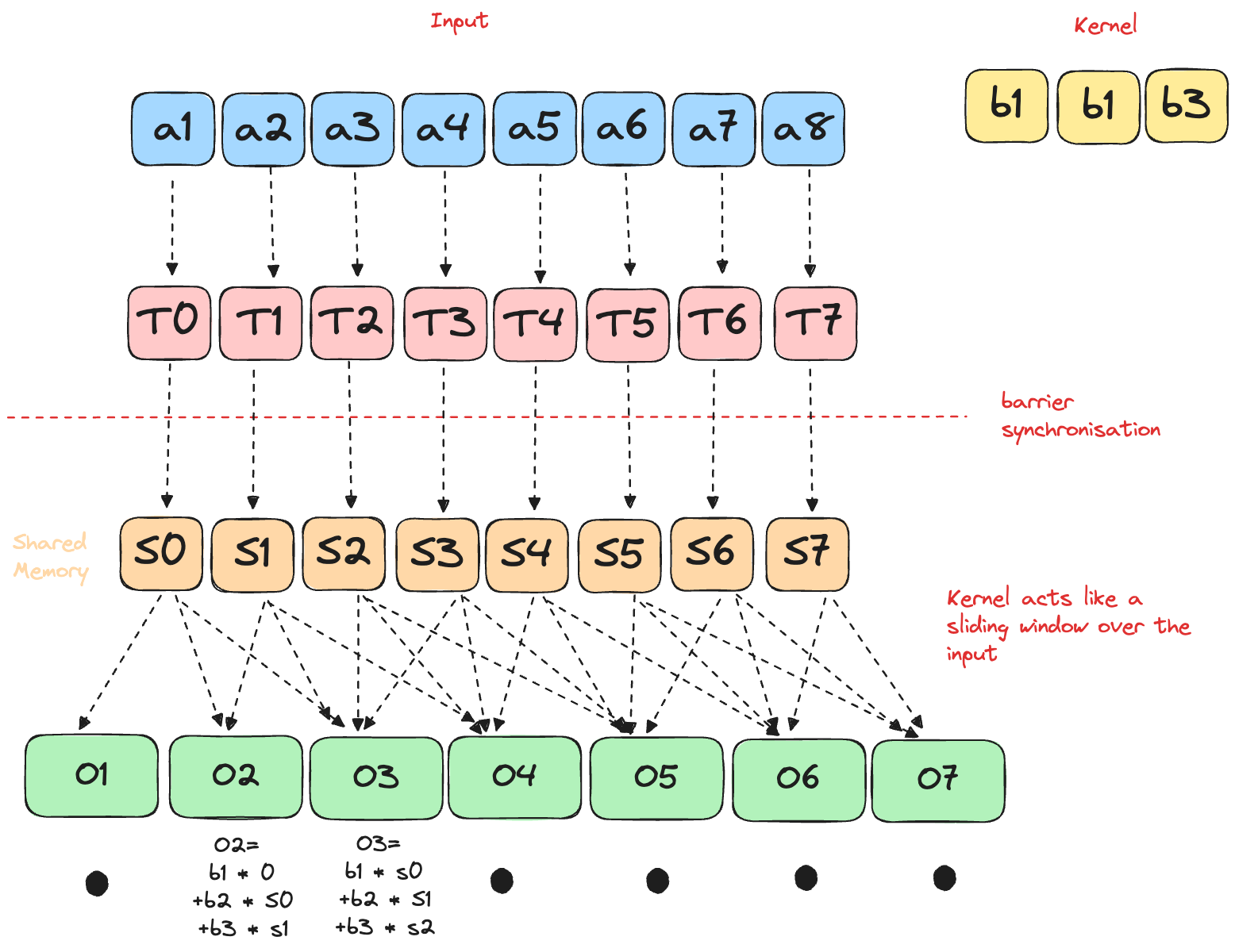
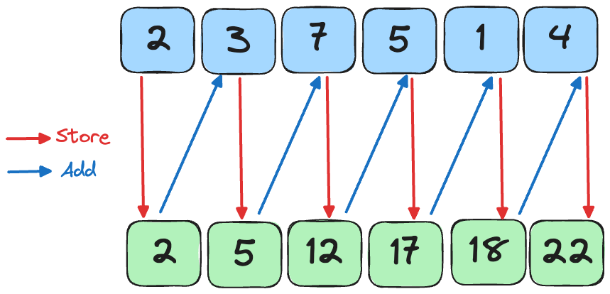
This puzzle is a bit different compared to traditional pooling: Instead of having a “kernel”, each output element is the running sum of the all the elements in the current window.
Solution
p09.mojo
alias TPB = 8
alias SIZE = 8
alias BLOCKS_PER_GRID = (1, 1)
alias THREADS_PER_BLOCK = (TPB, 1)
alias dtype = DType.float32


fn pooling(
    out: UnsafePointer[Scalar[dtype]],
    a: UnsafePointer[Scalar[dtype]],
    size: Int,
):
    shared = stack_allocation[
        TPB,
        Scalar[dtype],
        address_space = AddressSpace.SHARED,
    ]()
    global_i = block_dim.x * block_idx.x + thread_idx.x
    local_i = thread_idx.x
    if global_i < size:
        shared[local_i] = a[global_i]

    barrier()

    if global_i < size:
        if local_i - 2 >= 0:
            out[global_i] = (
                shared[local_i - 2] + shared[local_i - 1] + shared[local_i]
            )
        elif local_i - 1 >= 0:
            out[global_i] = shared[local_i - 1] + shared[local_i]
        else:
            out[global_i] = shared[local_i]
pixi run p09
# out: HostBuffer([11.0, 11.0, 11.0, 11.0, 11.0, 11.0, 11.0, 11.0])
# expected: HostBuffer([11.0, 11.0, 11.0, 11.0, 11.0, 11.0, 11.0, 11.0])The LayoutTensor version is nearly identical to the Raw Memory approach, so we’ll omit the code here for brevity.
Puzzle 10: Dot Product
The Dot Product of two vectors \(a\) and \(b\) is defined as [1]:
\[ c = a \cdot b = \sum_{i=0}^{n-1} a_i b_i \]
Similar to the previous puzzles, we can implement the dot-product by copying data to the shared memory, and running our operations on it.
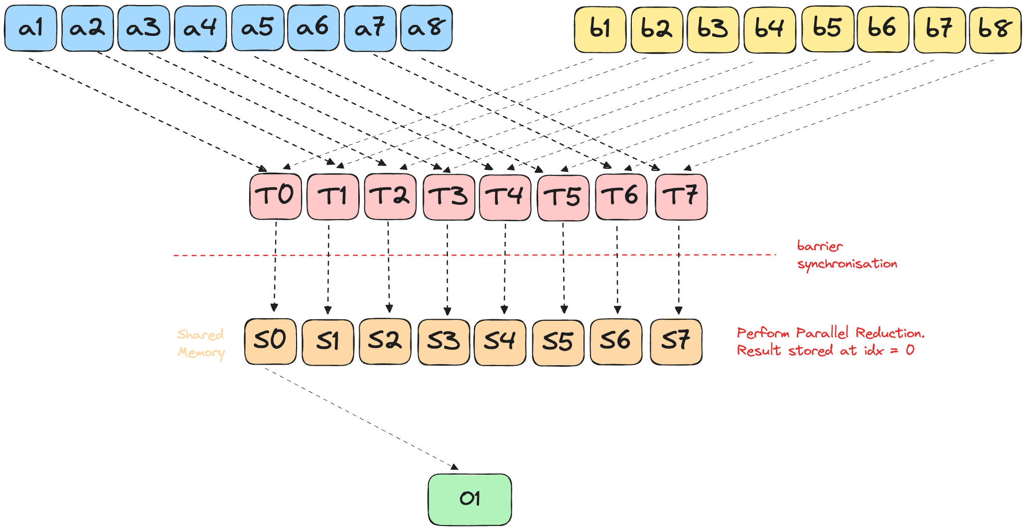
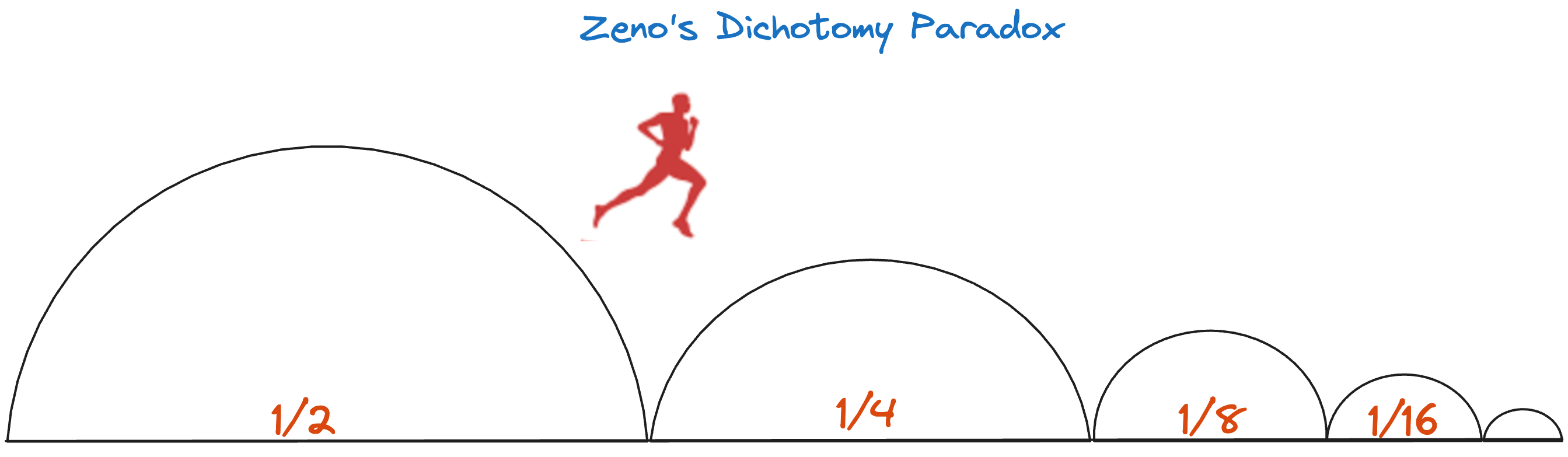
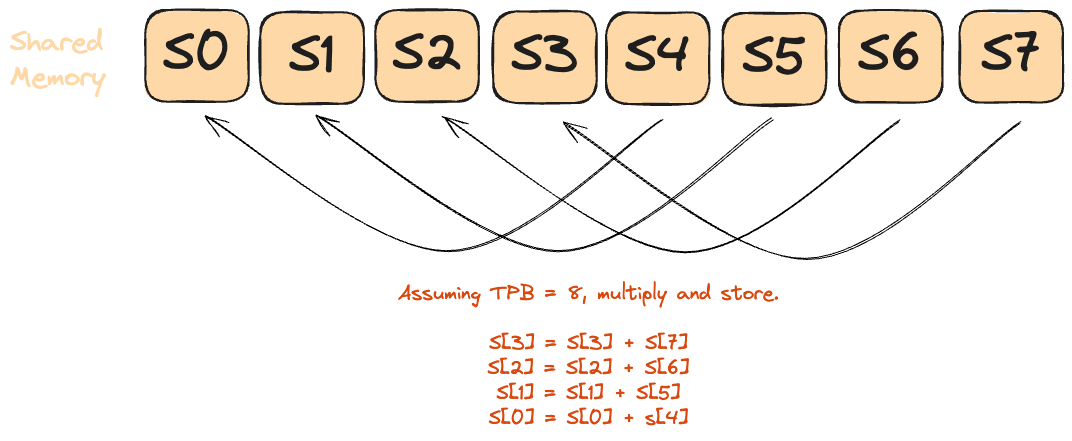
To implement dot product efficiently on a GPU, we will use parallel reduction. This is a classic pattern for aggregating values (sum, min, max, etc.) across a large array using many threads.
Picture Zeno’s “half-way” paradox [2]: you keep halving the leftover distance until you’re done. A parallel reduction does the same-each round halves the number of active threads instead of the distance. Unlike Zeno’s infinite halvings though, we stop at a concrete point: when only thread 0 remains active (stride becomes 0).
- Every thread multiplies its assigned
aandbelements and writes the partial product into shared memory. - Each reduction round:
- The active-thread count is cut in half (
stride /= 2). - Each surviving thread adds its value to the partner
stridepositions away. - A
barrier()guarantees all writes land before the next “half-step.”
- The active-thread count is cut in half (
- After log₂ (n) halvings, Zeno’s finish line is crossed-thread 0 alone holds the final dot-product.
This pattern is fast, highly parallel, and used everywhere in GPU programming for reductions (sum, min, max, etc).
Raw Memory
Solution
p10.mojo
fn dot_product(
    output: UnsafePointer[Scalar[dtype]],
    a: UnsafePointer[Scalar[dtype]],
    b: UnsafePointer[Scalar[dtype]],
    size: Int,
):
    global_idx = block_dim.x * block_idx.x + thread_idx.x
    local_idx = thread_idx.x
    if global_idx < size:
        shared[local_idx] = a[global_idx] * b[global_idx]

    barrier()

    stride = TPB // 2
    while(stride > 0):
        if local_idx < stride:
            shared[local_idx] += shared[local_idx + stride]

        barrier()
        stride = stride // 2

    # only allow thread 0 to write result
    if local_idx == 0:
output[0] = shared[0]Note: Instead of doing the parallel reduction, we could also implement the solution using a loop:
-    stride = TPB // 2
-    while(stride > 0):
-        if local_idx < stride:
-            shared[local_idx] += shared[local_idx + stride]
-
-        barrier()
-        stride = stride // 2
-
-    # only allow thread 0 to write result
-    if local_idx == 0:
-        output[0] = shared[0]
+    if global_idx < size:
+        for idx in range(size):
+            output[0] = output[0] + shared[idx]
While this approach also gives the correct answer for this puzzle, it has multiple problems:
- Race conditions: Multiple threads would simultaneously try to update output[0] without synchronization, causing lost updates.
- Thread divergence: When threads in a warp take different execution paths (some running the loop, others not), the GPU must serialize execution, destroying parallelism.
- Redundant computation: Every qualifying thread would compute the exact same sum over the entire array, wasting compute resources.
- Memory bottleneck: Repeated atomic operations to the same memory location (output[0]) create severe contention.
LayoutTensor
Solution
p10.mojo
alias TPB = 8
alias SIZE = 8
alias BLOCKS_PER_GRID = (1, 1)
alias THREADS_PER_BLOCK = (SIZE, 1)
alias dtype = DType.float32
alias layout = Layout.row_major(SIZE)
alias out_layout = Layout.row_major(1)

fn dot_product[
    in_layout: Layout, out_layout: Layout
](
    output: LayoutTensor[mut=True, dtype, out_layout],
    a: LayoutTensor[mut=True, dtype, in_layout],
    b: LayoutTensor[mut=True, dtype, in_layout],
    size: Int,
):
    # Use LayoutTensorBuilder instead of stack_allocation
    shared = tb[dtype]().row_major[TPB]().shared().alloc()
    global_idx = block_dim.x * block_idx.x + thread_idx.x
    local_idx = thread_idx.x

    if global_idx < size:
        shared[local_idx] = a[global_idx] * b[global_idx]

    barrier()

    stride = TPB // 2
    while(stride > 0):
        if local_idx < stride:
            shared[local_idx] += shared[local_idx + stride]

        barrier()
        stride = stride // 2

    # only allow thread 0 to write result
    if local_idx == 0:
        output[0] = shared[0]
Puzzle 11: 1D Convolution
Picture sliding a magnifying glass along a long strip of film. That’s exactly what a 1-D convolution does to any 1-D signal-audio samples, DNA bases, even bytes of log data.
- The kernel (a small weight vector) glides over the sequence one step at a time (or more if you set stride > 1).
- At each stop it multiplies the local window by its weights, sums the result, and drops a single number into the output map.
- Stack layers and you grow the “what can I see at once?” window (the receptive field) without blowing up parameters.
Why bother?
- Speed: A conv layer is just a batched matrix-mul-GPU catnip.
- Locality first, context later: Early layers grab short-range patterns (phonemes, k-mers). Deeper layers stitch them into bigger motifs (words, promoters).
- Channels generalize it: You convolve along length, but for each input channel you keep separate weights, sum across channels, and spit out new feature maps. Same trick as 2-D CNNs, just flattened.
For a better picture, see Ayush’s blog[3] on convolutions.
The convolution operation can be defined as: \[ (input\_signal\_a * kernel\_b)[i] = \sum_{j=0}^{\text{kernel\_size}-1} input\_signal\_a[i + j] * kernel\_b[j] \tag{1}\]
Single Block with Shared Memory
For this version, we assume that we only have a single block, and both the input data and the kernel fit within a block.
The implementation is:
- Intialise shared memory for both the input and the kernel
- Load data in the shared memory, and use
barrier()to sync all threads before performing computations. - In a loop, multiple the value of input and kernel, and add to a local variable.
- Assign the local variable to the right output index.
Solution
p11.mojo
alias TPB = 8
alias SIZE = 6
alias CONV = 3
alias BLOCKS_PER_GRID = (1, 1)
alias THREADS_PER_BLOCK = (TPB, 1)
alias dtype = DType.float32
alias in_layout = Layout.row_major(SIZE)
alias out_layout = Layout.row_major(SIZE)
alias conv_layout = Layout.row_major(CONV)


fn conv_1d_simple[
    in_layout: Layout, out_layout: Layout, conv_layout: Layout
](
    output: LayoutTensor[mut=False, dtype, out_layout],
    a: LayoutTensor[mut=False, dtype, in_layout],
    b: LayoutTensor[mut=False, dtype, conv_layout],
):
    global_i = block_dim.x * block_idx.x + thread_idx.x
    local_i = thread_idx.x
    # This is oversized! I've explained it later :)
    shared_a = tb[dtype]().row_major[TPB]().shared().alloc()
    shared_b = tb[dtype]().row_major[TPB]().shared().alloc()

    # This can also be optimised, as shown later.
    if global_i < SIZE:
        shared_a[local_i] = a[global_i]
        shared_b[local_i] = b[global_i]


    barrier()

    if global_i < SIZE:

        # Ensure the local var has the same type as the output
        # to avoid type casting errors.
        var local_sum: output.element_type = 0

        # Perform loop unrolling.
        @parameter
        for j in range(CONV):
            if local_i + j < SIZE:
                local_sum += shared_a[local_i + j] * shared_b[j]

        output[global_i] = local_sum
I deliberately allocate shared_a and shared_b with the block width (TPB) instead of the input length (SIZE) and filter length (CONV). The extra space isn’t needed for correctness-the kernel only touches the first SIZE/CONV elements-but it nicely demonstrates LayoutTensor’s masking: out-of-range indices are silently ignored. This trick keeps the buffer shape uniform across puzzles without cluttering the code with edge-case branches. The flip side is a bit of wasted shared memory, which can pinch if your kernel is already pushing the SRAM limit.
The optimal allocation of shared memory would be:
-    shared_a = tb[dtype]().row_major[TPB]().shared().alloc()
-    shared_b = tb[dtype]().row_major[TPB]().shared().alloc()
+    # Allocate exactly SIZE elements -> smaller shared-mem footprint
+    shared_a = tb[dtype]().row_major[SIZE]().shared().alloc()
+    # Allocate exactly CONV elements -> smaller shared-mem footprint
+    shared_b = tb[dtype]().row_major[CONV]().shared().alloc()
...

-    if global_i < SIZE:
-        shared_a[local_i] = a[global_i]
-        shared_b[local_i] = b[global_i]
+    if global_i < SIZE:
+        shared_a[local_i] = a[global_i]
+    if global_i < CONV:
+        shared_b[local_i] = b[global_i]
Loop Unrolling
@parameter is Mojo’s implementation of loop unrolling. This has the same functionality as pragma unroll(N) in CUDA.
When unroll is in effect, the optimizer determines and applies the best unrolling factor for each loop; in some cases, the loop control might be modified to avoid unnecessary branching. The compiler remains the final arbiter of whether the loop is unrolled[4].
@parameter isn’t limited to loops/branches-you can slap it on an inner function and Mojo will build a parametric closure, defined as[5]:
A parametric closure is a nested function decorated with
@parameter. Any values it captures from the surrounding scope are treated as compile-time constants. The compiler materialises one specialised version of the closure for every distinct set of captured values
Example:
parametric_closure.mojo
fn make_shift(off: Int):
    @parameter            # ← specialised per ‘off'
    fn shift(x: Int) -> Int:
        return x + off
    return shift

let s1 = make_shift(1)    # emits shift-$off=1
let s4 = make_shift(4)    # emits shift-$off=4
No runtime captures, no heap boxing-the constant off is literally spliced into the generated IR, so calls to s1/s4 inline like normal code and can be further unrolled or constant-folded.
Why is this safe? Mojo’s origin system[6] assigns each compile-time constant its own immutable origin. The closure therefore can’t outlive or mutate the thing it captured; once the surrounding scope ends those origins die too, guaranteeing that the specialised code never touches expired storage.
In summary, you get closure ergonomics plus “zero-cost abstraction”[7] performance-ideal for GPU kernels where every cycle and register matters.
Block Boundary
We now aim to perform convolution over an input that is larger than a single block. Due to the nature of convolution operation, this introduces interesting boundary conditions. Specifically, the output of block N now depends on block N - 1, when N > 1.
The blue cells are the data owned by the current thread-block. The orange cells are the first few elements of the next block that the convolution window will inevitably peek at.
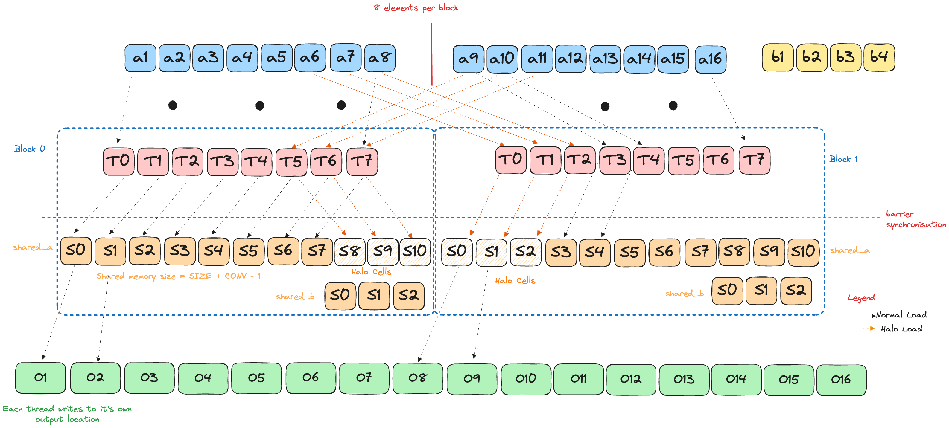
Problem statement
Run a 1-D convolution with a CONV₂-tap kernel over an input that is longer than one block (TPB threads). We want every thread to:
- Pull data from shared memory only (once it’s loaded, stay in-block)
- Avoid divergent branches and random global reads
- Keep the load pattern fully coalesced
Naïve global loads meet none of those goals-once a window crosses the block edge the tail threads must issue conditional, straggling reads (i.e. each thread grabs a lone, scattered element from global memory instead of part of one tidy, coalesced burst).
The halo idea
Give each block an in-block “fence extension”:
shared_a = …[TPB + (CONV₂ − 1)] # main slice + haloThe extra (CONV₂ − 1) slots-the halo-mirror the first (CONV₂ − 1) elements of the next block (or zeros if we’re already at EOF). That single change guarantees that every sliding window lives in one contiguous span of shared memory.
The elements that are involved in multiple tiles and loaded by multiple blocks are commonly referred to as halo cells or skirt cells since they “hang” from the side of the part that is used solely by a single block[8].
Loading recipe (matches the numbered arrows in the figure):
- Bulk copy - all
TPBthreads dump their element:
shared_a[t] = a[blockStart + t] - Halo fill - threads
t < (CONV₂ − 1)copy the tail:
shared_a[TPB + t] = (a[blockStart + TPB + t] if in-range else 0) - Kernel stash - threads
t < CONV₂cache the weights:
shared_b[t] = b[t] barrier()- everyone syncs
After step 4 every thread sees:
      main slice              halo
[ … local_i … TPB − 1 | TPB … TPB+CONV₂−2 ]
Code to perform the actual computation is the same as in Puzzle 10.
One barrier, no branches and 100 % shared-memory hits ensure our kernel is fast and efficient!
Solution
p11_block_boundary.mojo
alias SIZE_2 = 15
alias CONV_2 = 4
alias BLOCKS_PER_GRID_2 = (2, 1)
alias THREADS_PER_BLOCK_2 = (TPB, 1)
alias in_2_layout = Layout.row_major(SIZE_2)
alias out_2_layout = Layout.row_major(SIZE_2)
alias conv_2_layout = Layout.row_major(CONV_2)

fn conv_1d_block_boundary[
    in_layout: Layout, out_layout: Layout, conv_layout: Layout, dtype: DType
](
    output: LayoutTensor[mut=False, dtype, out_layout],
    a: LayoutTensor[mut=False, dtype, in_layout],
    b: LayoutTensor[mut=False, dtype, conv_layout],
):
    global_i = block_dim.x * block_idx.x + thread_idx.x
    local_i  = thread_idx.x

    # input slice + halo
    shared_a = tb[dtype]().row_major[TPB + CONV_2 - 1]().shared().alloc()

    # load kernel
    shared_b = tb[dtype]().row_major[CONV_2]().shared().alloc()

    if global_i < SIZE_2:
        # coalesced load of main slice
        shared_a[local_i] = a[global_i]

    # only first CONV_2 threads participate
    if local_i < CONV_2:
        # load kernel into shared memory
        shared_b[local_i] = b[local_i]

    # threads responsible for halo load
    if local_i < CONV_2 - 1:
        # element that lives in next block
        var next_idx = global_i + TPB
        # pad with zeros
        shared_a[local_i + TPB] = a[next_idx] if next_idx < SIZE_2 else 0.0

    barrier()

    # skip threads mapping past the end
    if global_i < SIZE_2:
        var local_sum: output.element_type = 0.0

        @parameter
        for j in range(CONV_2):
            # dot product of window & kernel
            local_sum += shared_a[local_i + j] * shared_b[j]
        output[global_i] = local_sum
pixi run p11 --block-boundary
# out: HostBuffer([14.0, 20.0, 26.0, 32.0, 38.0, 44.0, 50.0, 56.0, 62.0, 68.0, 74.0, 80.0, 41.0, 14.0, 0.0])
# expected: HostBuffer([14.0, 20.0, 26.0, 32.0, 38.0, 44.0, 50.0, 56.0, 62.0, 68.0, 74.0, 80.0, 41.0, 14.0, 0.0])From 1D Strips to 2D Tiles
Sliding a 1D window over an audio buffer was straightforward: one axis, one index. Images and matrices, however, live on chessboards, not lines. To convolve or multiply them efficiently we need to map two spatial dimensions onto the GPU’s grid-block-thread hierarchy.
Thread Hierarchy in 2D
The GPU execution model extends naturally to 2D with a three-level hierarchy:
| Level | Analogy | Coordinates |
|---|---|---|
| Grid | City | (blockIdx.x, blockIdx.y) |
| Block | City block | (threadIdx.x, threadIdx.y) |
| Thread | House | computed from block + thread IDs |
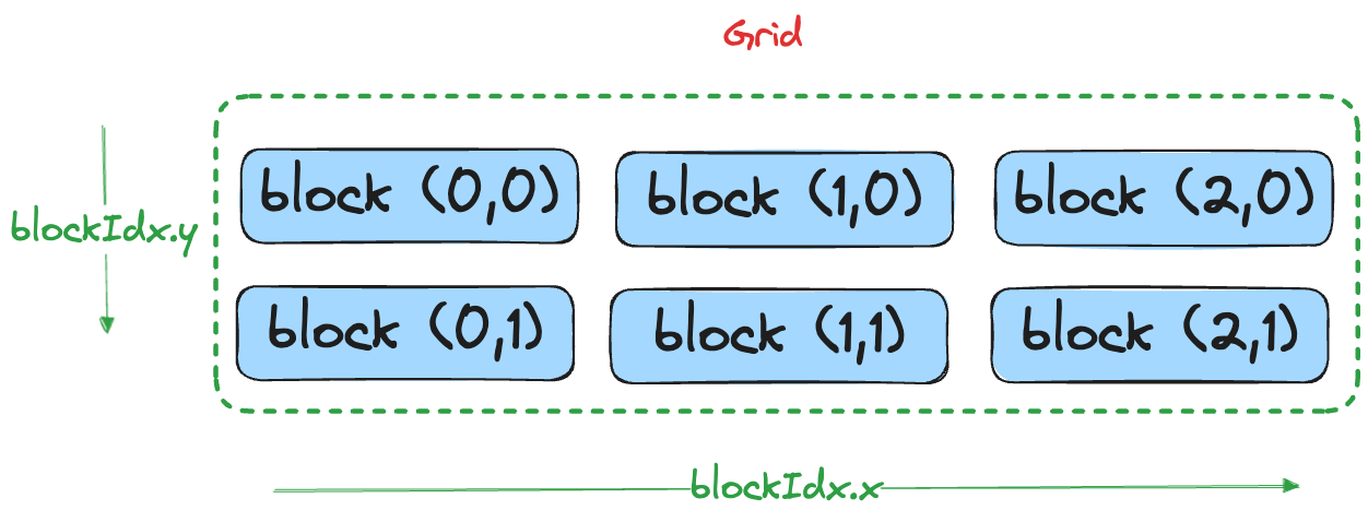
Within each block, you choose the thread footprint at kernel launch with THREADS_PER_BLOCK = (blockDim.x, blockDim.y), giving blockDim.x * blockDim.y total threads per block.
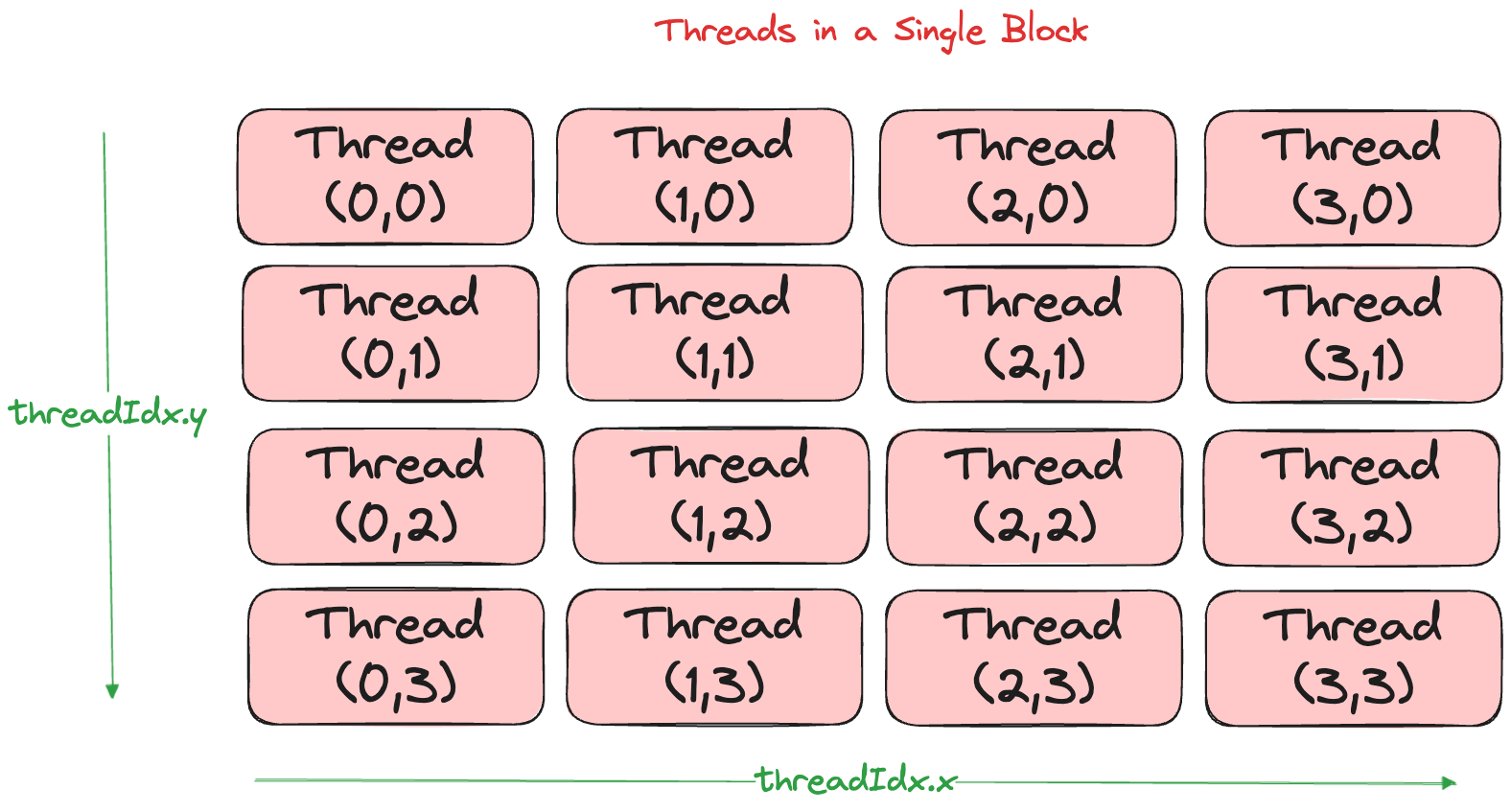
What’s a Warp?
Under the hood, the GPU executes 32 threads at once in groups called warps (AMD calls them wavefronts[9]). All 32 lanes run the same instruction each cycle (SIMT). Thread divergence or uncoalesced memory access forces the warp to serialize, so we design our 2D tiles around these 32-lane chunks.
Hardware facts:
- SIMT execution: All 32 threads in a warp execute the same instruction. Branching splits the warp and runs paths serially.
- Memory coalescing: A warp performs one 32-lane memory request when threads access consecutive addresses.
- Occupancy: The number of warps that can run simultaneously on a streaming multiprocessor, limited by registers and shared memory per block.
Grids and blocks are a programmer-friendly abstraction. Warps are what the hardware actually schedules.
Computing Global Matrix Indices
The key insight is that every thread computes its global position using the same formula:
let col = block_idx.x * block_dim.x + thread_idx.x  # column index
let row = block_idx.y * block_dim.y + thread_idx.y  # row index
This maps the thread hierarchy directly to matrix coordinates:
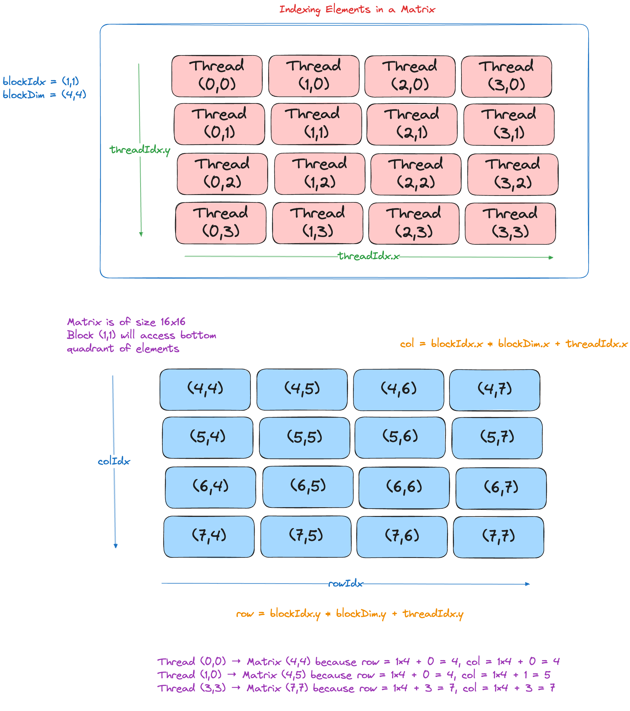
For an M×N output matrix, you typically launch:
alias TILE_X = 16  # threads per block in x dimension
alias TILE_Y = 16  # threads per block in y dimension
alias BLOCKS_X = ceildiv(N, TILE_X)  # columns
alias BLOCKS_Y = ceildiv(M, TILE_Y)  # rows
alias BLOCKS_PER_GRID = (BLOCKS_X, BLOCKS_Y)
alias THREADS_PER_BLOCK = (TILE_Y, TILE_X)
Choosing Tile Size
As shown earlier, because a warp wants contiguous addresses, we’ll carve the matrix into 16×16 tiles. Here’s how the hardware facts translate to design choices:
- Warp-aligned rows: Make tile width a multiple of 32 (warp size) so each row loads as a single coalesced burst.
- Shared memory reuse: Square tiles minimize the halo-to-area ratio, so each global load gets reused ~K times across the convolution window.
- Resource budgeting: 256-512 threads per block (8-16 warps) keeps enough warps resident for latency hiding without exhausting registers or shared memory.
A 16×16 tile gives 256 threads = 8 warps, hitting the sweet spot for most GPUs.
Bounds Checking
Since matrix dimensions are rarely exact multiples of tile size, always guard against out-of-bounds access:
if row < M and col < N:
    # safe to access matrix[row, col]
Mojo doesn’t provide automatic bound checking when writing to shared memory [10].
Worked Example: 40×50 Matrix with 16×16 Tiles
For a 40×50 matrix with 16×16 tiles:
        col 0……15 16……31 32……47
 row
 0…15    Blk(0,0)  Blk(1,0)  Blk(2,0)
16…31    Blk(0,1)  Blk(1,1)  Blk(2,1)
32…39    Blk(0,2)  Blk(1,2)  Blk(2,2)
Each thread in Block(1,1) computes one element where row ∈ [16,31] and col ∈ [16,31]. Note that Block(2,2) only processes 8×16 elements due to the matrix boundaries.
Indexing Pattern Template
let row = block_idx.y * block_dim.y + thread_idx.y
let col = block_idx.x * block_dim.x + thread_idx.x
if row < M and col < N:
    # Process matrix[row, col]
This indexing pattern appears in every 2D GPU kernel-matrix multiplication, 2D convolution, transpose, etc.
Note: Mojo/CUDA grids and blocks can also have a third dimension (
block_idx.z,thread_idx.z) for problems like 3D volume processing or batch operations. We’ll cover that when we encounter 3D kernels.
Bonus: 2D Convolution
We can extend our implementation for 1D convolution to a 2D convolution.
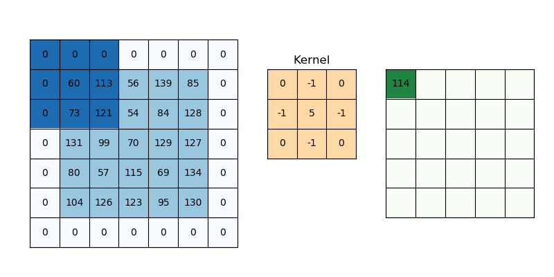
Everything is exactly the same idea as 1-D, only now we have two spatial dims:
- We launch a 2D grid of
(ceildiv(WIDTH,TPB_Y), ceildiv(HEIGHT,TPB_X))blocks ofTPB_Y×TPB_Xthreads. - Each block allocates a shared tile of size
(TPB_Y+K−1)×(TPB_X+K−1)to hold its “main” patch plus a one‐pixel halo on the bottom/right. - We also stash the full
K×Kkernel into shared_k. - After a single barrier(), each thread does two nested
@parameterloops overky,kx∈[0,K)to compute a dot‐product.
Solution
p11_conv_2d.mojo
from math import ceildiv
...

alias TPB_X = 8
alias TPB_Y = 8
alias WIDTH = 16
alias HEIGHT = 12
alias K     = 3
alias BLOCKS_PER_GRID_2D  = (ceildiv(WIDTH, TPB_Y),  ceildiv(HEIGHT, TPB_X))
alias THREADS_PER_BLOCK_2D = (TPB_Y, TPB_X)

fn conv_2d_halo[
    in_layout : Layout, out_layout : Layout,
    k_layout  : Layout, dtype : DType
](
    output : LayoutTensor[mut=False, dtype, out_layout],
    inp    : LayoutTensor[mut=False, dtype, in_layout],
    kernel : LayoutTensor[mut=False, dtype, k_layout],
):
    let gx = block_idx.x * block_dim.x + thread_idx.x
    let gy = block_idx.y * block_dim.y + thread_idx.y
    let lx = thread_idx.x
    let ly = thread_idx.y

    const TILE_W = TPB_X + K - 1
    const TILE_H = TPB_Y + K - 1

    # allocate (main + halo) + kernel
    shared_img = tb[dtype]().row_major[TILE_H, TILE_W]().shared().alloc()
    shared_k   = tb[dtype]().row_major[K,K]().shared().alloc()

    # 1) bulk copy
    if gx < WIDTH && gy < HEIGHT:
        shared_img[ly, lx] = inp[gy, gx]
    else:
        shared_img[ly, lx] = 0.0

    # 2) halo copy (strided so we cover the whole TILE_H/TILE_W)
    var hy = ly
    while hy < TILE_H:
        var hx = lx
        let gy2 = block_idx.y * block_dim.y + hy
        while hx < TILE_W:
            let gx2 = block_idx.x * block_dim.x + hx
            shared_img[hy, hx] = (
                inp[gy2, gx2] if (gy2 < HEIGHT && gx2 < WIDTH) else 0.0
            )
            hx += TPB_X
        hy += TPB_Y

    # 3) stash the kernel
    if ly < K && lx < K:
        shared_k[ly, lx] = kernel[ly, lx]

    barrier()  # sync both shared buffers

    # 4) compute 3×3 dot‐product
    if gx < WIDTH && gy < HEIGHT:
        var local_sum: Float32 = 0.0
        @parameter
        for ky in range(K):
            @parameter
            for kx in range(K):
                local_sum += shared_img[ly + ky, lx + kx] * shared_k[ky, kx]
        output[gy, gx] = local_sum
After making a few changes to the test harness, we get the following result:
pixi run p11 --conv-2d
# out: HostBuffer([9.0, 9.0, 9.0, 9.0, 9.0,...,6.0, 3.0, 6.0, 6.0, 6.0, 6.0, 6.0, 6.0, 6.0, 6.0, 6.0, 6.0, 6.0, 6.0, 6.0, 6.0, 4.0, 2.0, 3.0, 3.0, 3.0, 3.0, 3.0, 3.0, 3.0, 3.0, 3.0, 3.0, 3.0, 3.0, 3.0, 3.0, 2.0, 1.0])
# expected: HostBuffer([9.0, 9.0, 9.0, 9.0, 9.0,..., 6.0, 6.0, 6.0, 6.0, 6.0, 6.0, 6.0, 6.0, 6.0, 6.0, 6.0, 6.0, 6.0, 6.0, 4.0, 2.0, 3.0, 3.0, 3.0, 3.0, 3.0, 3.0, 3.0, 3.0, 3.0, 3.0, 3.0, 3.0, 3.0, 3.0, 2.0, 1.0])
We’ll dive into the shared memory tricks like parking partial results, handling 2-D thread and block indexing, and performing halo copies when we get to matrix multiply in Puzzle 14.
Puzzle 12: Prefix Sum
The prefix sum (or scan) problem takes an input array [a₀, a₁, …, aₙ₋₁] and produces the running totals
[a₀, (a₀ ⊕ a₁), …, (a₀ ⊕ a₁ ⊕ … ⊕ aₙ₋₁)]It’s a foundational primitive in parallel computing-used for stream compaction, sorting, histograms, and more. At first glance, prefix sum looks inherently serial (each output depends on all previous inputs), but clever algorithms can parallelize it efficiently.
Hillis-Steele Algorithm
A straightforward parallel scan is the Hillis-Steele approach: at each distance d = 1, 2, 4, … every element adds in the value from d positions back. This is the same as the method shown in Puzzle 10
# inclusive scan, power-of-two length
def hillis_steele_scan(a, ⊕):
    n = len(a)
    temp = a.copy()
    d = 1
    while d < n:
        for i in range(n):
            temp[i] = a[i] if i < d else a[i - d] ⊕ a[i]
        a, temp = temp, a
        d *= 2
    return a
In Mojo, this looks as follows:
Solution
p12_simple.mojo
fn prefix_sum_simple[
    layout: Layout
](
    output: LayoutTensor[mut=False, dtype, layout],
    a: LayoutTensor[mut=False, dtype, layout],
    size: Int,
):
    global_i = block_dim.x * block_idx.x + thread_idx.x
    local_i = thread_idx.x
    for idx in range(Int(log2(Scalar[dtype](TPB)))):
        if local_i >= offset and local_i < SIZE:
            shared[local_i] += shared[local_i - offset]

        barrier()
        offset *= 2

    if global_i < SIZE:
        output[global_i] = shared[local_i]
pixi run p12 --simple
# out: HostBuffer([0.0, 1.0, 3.0, 6.0, 10.0, 15.0, 21.0, 28.0])
# expected: HostBuffer([0.0, 1.0, 3.0, 6.0, 10.0, 15.0, 21.0, 28.0])Each of the log₂(n) rounds does up to n parallel additions (one per active element), so total work is \(\sum_k n = nlog(n)\). Because rounds are serialized by barriers, the longest dependency chain is one add per round i.e \(O(log n)\).
Blelloch’s Two‐Pass Algorithm
Blelloch’s two-pass scan does Θ(n) work by splitting the job into an up-sweep (build a reduction tree) and a down-sweep (propagate prefixes) [11].
Why prefer it over the classic Hillis-Steele (Algorithm 1)?
Hardware constraints: Hillis-Steele assumes one processor per element and updates the array in-place every round. A real GPU doesn’t grant that luxury: a “1024-thread” block actually runs in 32-thread warps that time-slice on the same SM. When warp 0 pauses and warp 1 resumes, in-place writes from one warp can overwrite data the other still needs.
Synchronisation cost: Avoiding the overwrite requires a barrier after every addition - log₂(n) rounds × n threads ⇒ Θ(n log n) operations plus all those barriers.
Blelloch’s fix to these problems is to break the up-sweep and down-sweep into separate phases:
- Up-sweep and down-sweep touch disjoint tree levels, so threads never trample each other within a phase.
- Only two global barriers are needed (one between the phases, one at the end).
- Now you get Θ(n) work and correctness, even for arrays much bigger than a warp.
The result is a scan that is both faster and safer on modern GPUs.
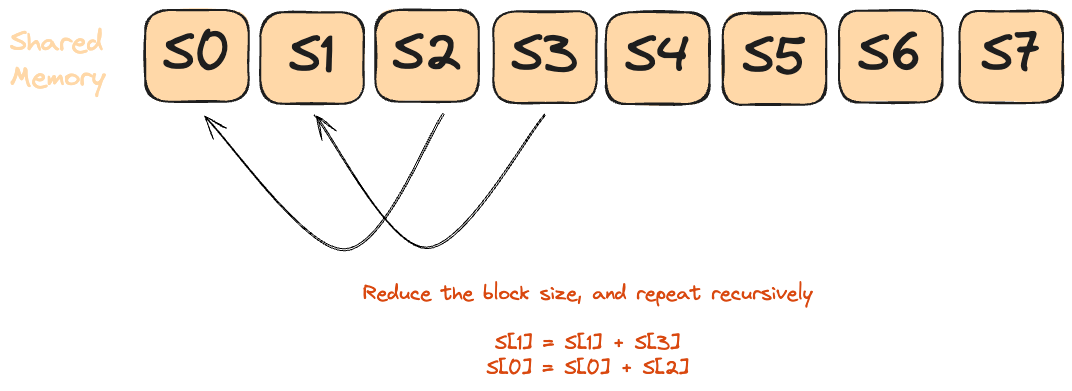
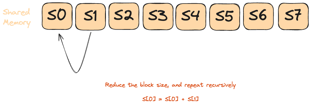
Up-sweep (reduce)
- Build a binary reduction tree over log₂(n) rounds:
- Round 1 (step=1): sum each adjacent pair, storing results at indices 1, 3, 5, …
- Round 2 (step=2): merge those partial sums into blocks of 4, writing into indices 3, 7, 11, …
- Continue doubling the span each round until step = n/2
- After the final round, a[n-1] holds the overall total
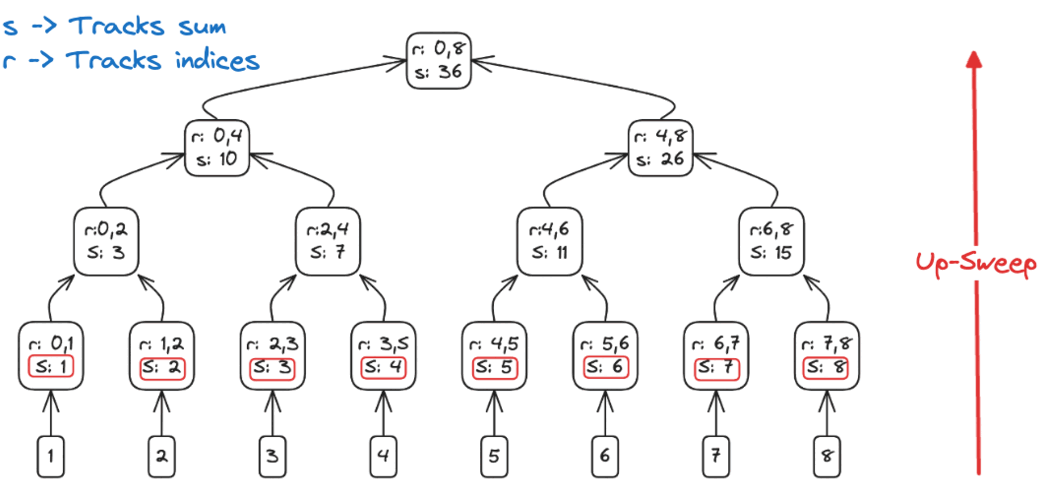 Up-Sweep: combining elements in a binary-tree fashion-build partial sums until the final element holds the total.
Down-sweep (propagate)
After the up-sweep leaves a[n-1] containing the overall sum, we walk the tree top-down to scatter prefix sums into every slot:
- Initialize the down-sweep with a window size of
step = n/2.
- Loop as long as
step >= 1:- Partition the array into blocks of size
2*step. For each block starting at indexi:- Temporarily store the left-child total from
a[i + step - 1].
- Overwrite that left slot with the right-child subtotal from
a[i + 2*step - 1].
- Add the saved left-child total to the right slot, giving the correct prefix for that subtree.
- Temporarily store the left-child total from
- Issue a
barrier()so all threads sync before shrinking the window.
- Halve the window:
step = step / 2.
- Partition the array into blocks of size
- With each pass, the partial sums trickle down one level of the binary tree; after log₂(n) iterations every element holds its exclusive prefix sum.
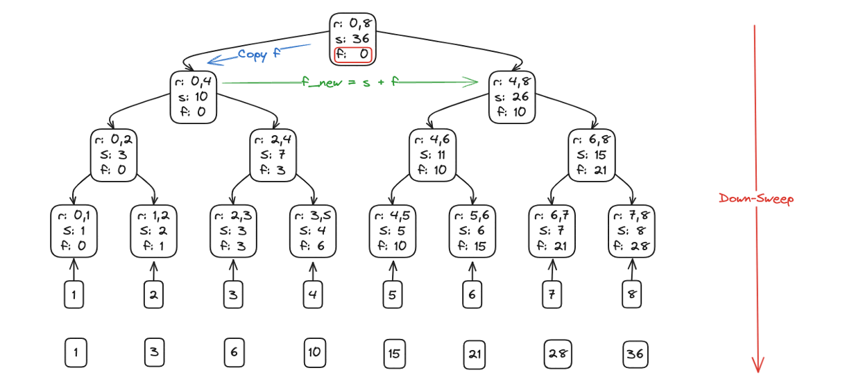
Down Sweep: siblings swap and accumulate, driving the scan from root back to leaves.
Total Operations: \(\Theta(n)\), parallel depth: \(\Theta(\log_2 n)\).
Solution (Blelloch up-sweep + down-sweep)
p12_blelloch.mojo
fn prefix_sum_blelloch[
    layout: Layout
](
    output:   LayoutTensor[mut=True, dtype, layout],
    a:     LayoutTensor[mut=False, dtype, layout],
    size:  Int,
):
    global_idx = block_idx.x*block_dim.x + thread_idx.x
    local_idx = thread_idx.x
    shared = tb[dtype]().row_major[SIZE]().shared().alloc()

    if global_idx < size:
        shared[local_idx] = a[global_idx]
    barrier()

    # Up-sweep
    var stride = 1
    while stride < size:
        step = stride * 2
        if (local_idx % step == step - 1) and (local_idx < size):
            shared[local_idx] += shared[local_idx - stride]
        barrier()
        stride = step

    # Down-sweep
    if local_idx == size - 1:
        shared[local_idx] = 0
    barrier()

    var half = stride >> 1
    while half > 0:
        step = half * 2
        if (local_idx % step == step - 1) and (local_idx < size):
            t = shared[local_idx - half]
            shared[local_idx - half] = shared[local_idx]
            shared[local_idx] += t
        barrier()
        half = half >> 1

    if global_idx < size:
        output[global_idx] = shared[local_idx] + a[global_idx]
pixi run p12 --blelloch
# out: HostBuffer([0.0, 1.0, 3.0, 6.0, 10.0, 15.0, 21.0, 28.0])
# expected: HostBuffer([0.0, 1.0, 3.0, 6.0, 10.0, 15.0, 21.0, 28.0])This is not the most efficient implementation, but I hope this provides some intuition about the algorithm!
Block Boundary
The key difference in this version is that now we have an input array that is larger than the size of a single block.
We split the global scan into two bite-sized passes:
Phase 1 - Local Scan
Each block copies its slice into shared memory.
Perform an in-block naive scan/Blelloch scan exactly as in the single-block case.
The last thread of the block stashes the block’s total after the scan into an auxiliary slot at the tail of
output:# |<--- SIZE_2 --->|<-- #blocks -->| # [ prefix sums ][ block totals ]
Phase 2 - Propagate block totals
- Every thread grabs the aggregate from the previous block (
totals[block_id-1]) and adds it to its own prefix.
Now every element holds the inclusive scan over the whole array.
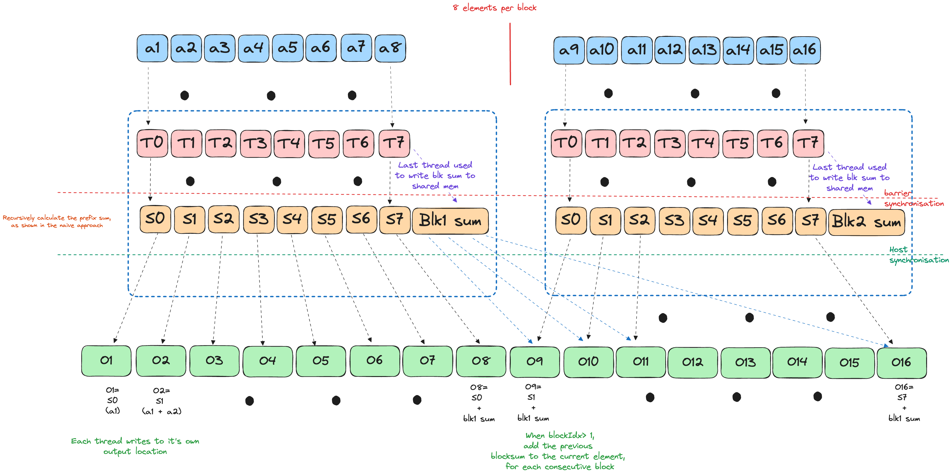
We launch the above phases as two separate kernels.
A host-side synchronisation sits between the launches. That call flushes the work queue and waits until Phase 1 has fully committed its writes to global memory, ensuring the per-block totals are complete and visible before Phase 2 starts consuming them. Skip the sync and the driver is free to overlap or reorder the kernels, letting Phase 2 read garbage.
Solution (Block Boundary Version)
p12_block_boundary.mojo
fn prefix_sum_local_phase[
    out_layout: Layout, in_layout: Layout
](
    output: LayoutTensor[mut=False, dtype, out_layout],
    a: LayoutTensor[mut=False, dtype, in_layout],
    size: Int,
):
    global_i = block_dim.x * block_idx.x + thread_idx.x
    local_i = thread_idx.x
    shared = tb[dtype]().row_major[EXTENDED_SIZE]().shared().alloc()

    if global_i < SIZE_2:
        shared[local_i] = a[global_i]

    barrier()
    offset = 1

    for idx in range(Int(log2(Scalar[dtype](TPB)))):
        if local_i >= offset and local_i < SIZE_2:
            shared[local_i] += shared[local_i - offset]

        barrier()
        offset *= 2

    if global_i < SIZE_2:
        output[global_i] = shared[local_i]

    if local_i == TPB - 1:
        output[size + block_idx.x] += shared[local_i]


# Kernel 2: Add block sums to their respective blocks
fn prefix_sum_block_sum_phase[
    layout: Layout
](output: LayoutTensor[mut=False, dtype, layout], size: Int):
    global_i = block_dim.x * block_idx.x + thread_idx.x
    # FILL ME IN (roughly 3 lines)
    if block_idx.x > 0 and global_i < size:
        prev_block_sum = output[SIZE_2 + block_idx.x - 1]
        output[global_i] += prev_block_sum
pixi run p12
# out: HostBuffer([0.0, 1.0, 3.0, 6.0, 10.0, 15.0, 21.0, 28.0, 36.0, 45.0, 55.0, 66.0, 78.0, 91.0, 105.0, 28.0, 77.0]) # last 2 elements are the block sums
# expected: HostBuffer([0.0, 1.0, 3.0, 6.0, 10.0, 15.0, 21.0, 28.0, 36.0, 45.0, 55.0, 66.0, 78.0, 91.0, 105.0])Puzzle 13: Axis Sum
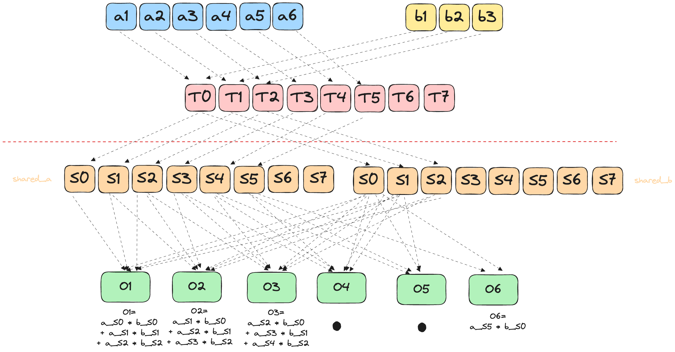
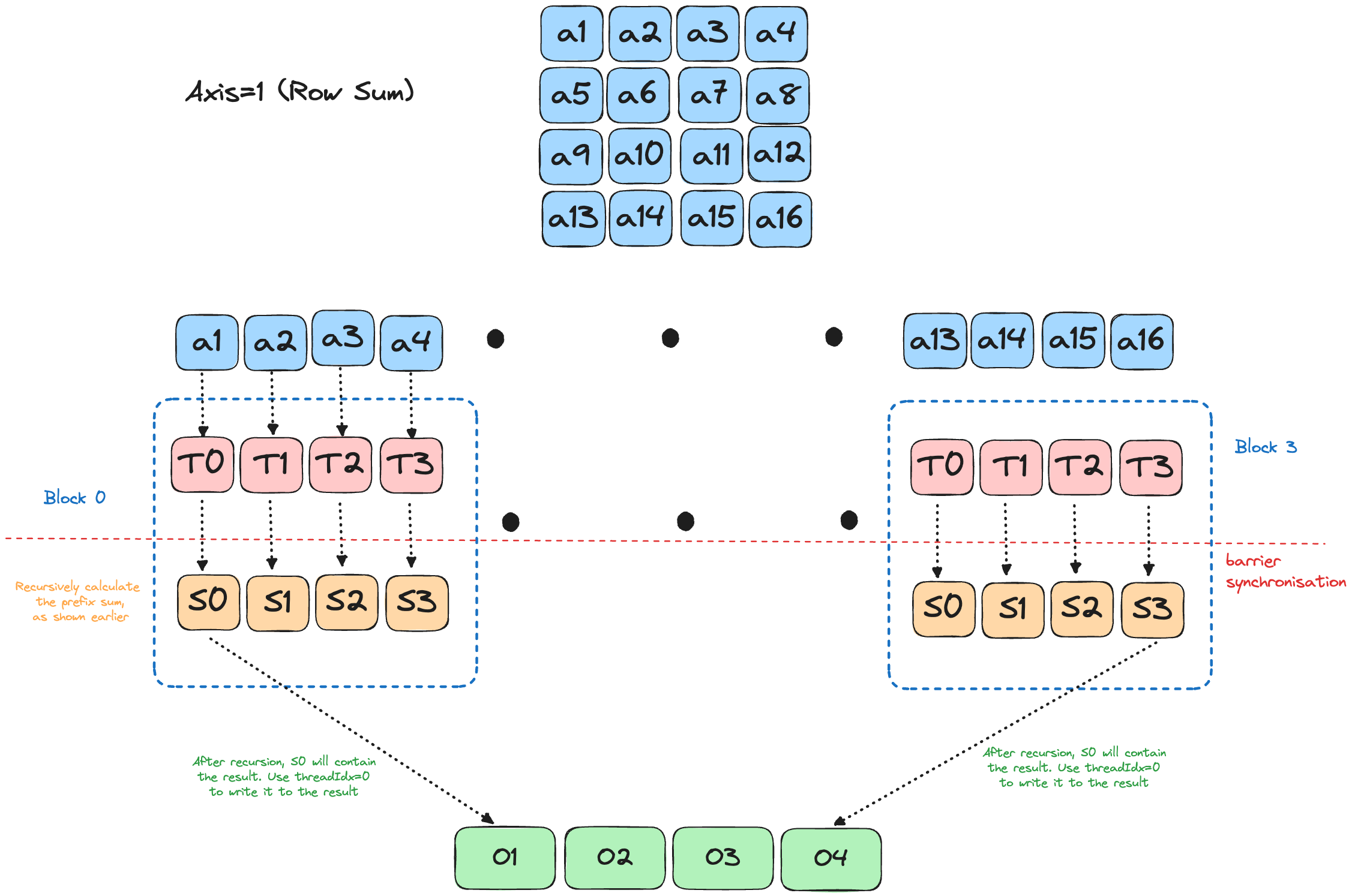
Axis sum is the 2-D sibling of the dot‐product/prefix puzzles: take a matrix A and collapse one dimension by summing over it.
\[ \begin{aligned} \text{axis}=0 &\;\Longrightarrow\; \text{column-sum:}\;\; out[j] & = \sum_{k} A_{k,j}, \qquad j = 0,\dots,N-1 \\[4pt] \text{axis}=1 &\;\Longrightarrow\; \text{row-sum:}\;\; out[i] & = \sum_{k} A_{i,k}, \qquad i = 0,\dots,M-1 \end{aligned} \]
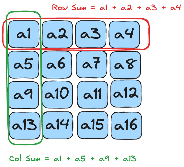
Each row/column is an embarrassingly-parallel reduction, so the GPU kernel just assigns one warp (or block) per slice and performs a standard shared-memory reduction inside the slice.
Solution
p13.mojo
fn axis_sum[
    in_layout: Layout, out_layout: Layout
](
    output: LayoutTensor[mut=False, dtype, out_layout],
    a: LayoutTensor[mut=False, dtype, in_layout],
    size: Int,
):
    local_i = thread_idx.x
    batch = block_idx.y
    shared = tb[dtype]().row_major[TPB]().shared().alloc()

    if local_i < SIZE:
        shared[local_i] = a[batch, local_i]

    barrier()

    var stride = TPB // 2
    while stride > 0:
        if local_i < stride and local_i + stride < SIZE:
            shared[local_i] += shared[local_i + stride]
        barrier()
        stride //= 2

    # Use first thread to write result
    if local_i == 0:
        # Output shape is [batch_size, 1]
        # which we why we need the last dimension
        output[batch, 0] = shared[0]
pixi run p13We can also perform column-sum(axis=0) with a trivial change:
-    if local_i < SIZE:
-        shared[local_i] = a[batch, local_i]
+    if local_i < SIZE:
+        shared[local_i] = a[local_i, batch]
Puzzle 14: Matmul
Arguably the single most important operation in GPU computing, the humble General Matrix Multiplication (GEMM) operation is the computational workhorse behind literally all deep learning models-from simple linear layers to massive transformer architectures.
\[ C_{i,j} = \sum_{k=1}^{K} A_{i,k} \cdot B_{k,j} \]
Requirement: For matrix multiplication \(C = AB\) to be valid, the number of columns in \(A\) must equal the number of rows in \(B\).
That is, if \(A\) is shape \((M, K)\) and \(B\) is shape \((K, N)\), then \(C\) will be shape \((M, N)\).
GEMM’s ubiquity stems from its perfect match with GPU architecture: thousands of independent multiply-add operations that can be parallelized across thousands of cores. Yet this apparent simplicity masks a deep optimization challenge. Memory bandwidth, cache hierarchies, and thread synchronization all conspire to make naive implementations crawl while hand-tuned libraries like cuBLAS achieve near-theoretical peak performance.
Matmul tuning is a rabbit hole - see Simon Boehm’s fantastic deep-dive [12] for how wild it gets.
For now, we’ll focus on the core techniques demonstrated by the official puzzle-shared memory tiling and thread cooperation-to build intuition for how high-performance GEMM kernels actually work.
Global Memory Version
Based on the 2D indexing section, each thread computes one C[row, col] by loading A[row, k] and B[k, col] from global memory, multiplying and accumulating over k. We unroll the k‐loop to cut loop overhead and boost throughput.
Solution
p14_naive.mojo
fn naive_matmul[
    layout: Layout, size: Int
](
    output: LayoutTensor[mut=False, dtype, layout],
    a: LayoutTensor[mut=False, dtype, layout],
    b: LayoutTensor[mut=False, dtype, layout],
):
    row = block_dim.y * block_idx.y + thread_idx.y
    col = block_dim.x * block_idx.x + thread_idx.x

    if row < SIZE and col < SIZE:
        # Need this to ensure the mojo compiler knows
        # the type of `running_sum`, otherwise it will
        # complain
        var running_sum: output.element_type = 0

        @parameter
        for k in range(SIZE):
            running_sum += a[row, k] * b[k, col]
        output[row, col] = running_sum
pixi run p14 --naive
# out: HostBuffer([4.0, 6.0, 12.0, 22.0])
# expected: HostBuffer([4.0, 6.0, 12.0, 22.0])Shared Memory Version
The previous version suffers from repeated global memory reads. We can optimize this using shared memory:
- Load matrix tiles once
- Synchronize threads
- Compute using the cached data.
Solution
p14_shared.mojo
fn single_block_matmul[
    layout: Layout, size: Int
](
    output: LayoutTensor[mut=False, dtype, layout],
    a: LayoutTensor[mut=False, dtype, layout],
    b: LayoutTensor[mut=False, dtype, layout],
):
    row = block_dim.y * block_idx.y + thread_idx.y
    col = block_dim.x * block_idx.x + thread_idx.x
    local_row = thread_idx.y
    local_col = thread_idx.x
    shared_a = tb[dtype]().row_major[TPB, TPB]().shared().alloc()
    shared_b = tb[dtype]().row_major[TPB, TPB]().shared().alloc()
    if row < size and col < size and local_row < size and local_col < size:
        shared_a[local_row, local_col] = a[row, col]
        shared_b[local_row, local_col] = b[row, col]

    barrier()
    if row < size and col < size and local_row < size and local_col < size:
        var running_sum: output.element_type = 0.0

        @parameter
        for k in range(size):
            running_sum += a[local_row, k] * b[k, local_col]

        output[row, col] = running_sum
pixi run p14 --naive
# out: HostBuffer([4.0, 6.0, 12.0, 22.0])
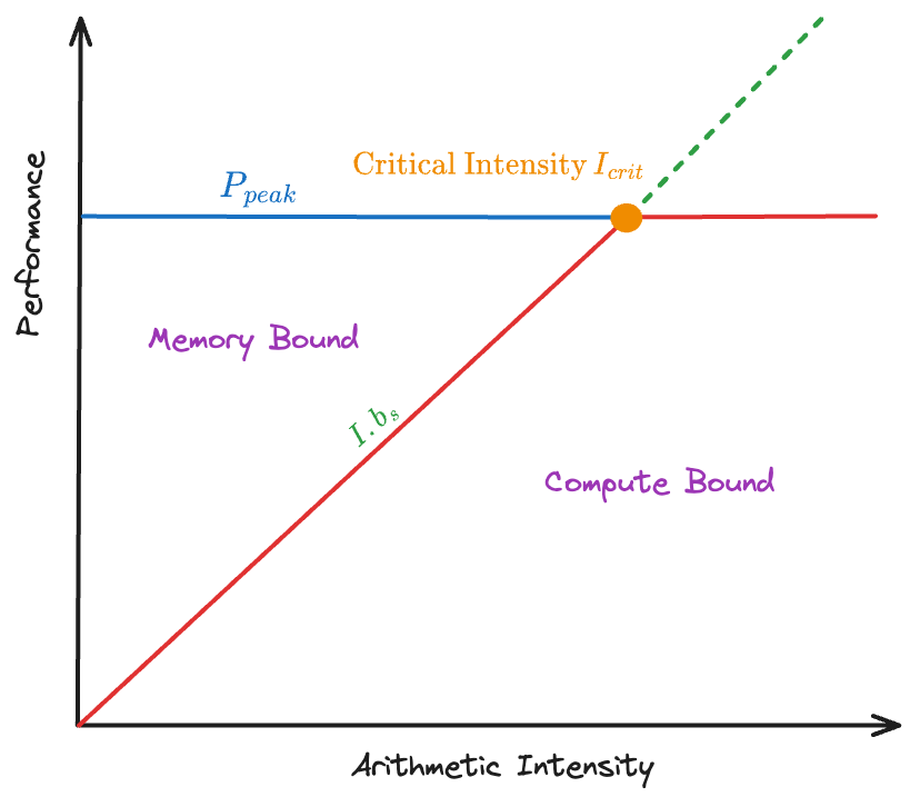
# expected: HostBuffer([4.0, 6.0, 12.0, 22.0])The Roofline Model offers a first-order answer to a GPU performance question: is my kernel limited by arithmetic throughput or by memory bandwidth?
It does so by plotting operational intensity (FLOPs per byte) against two ceilings - the hardware’s peak FLOP/s and peak DRAM bandwidth—so you can see at a glance which resource is the bottleneck.
Roofline Model
Note: The Modular GPU Puzzles guide already walks through the full roofline derivation, but we’ll repeat it here so that you can follow along without leaving this post.
The first step is abstracting the hardware-software complexity into a tractable model.
Hardware Model
Classic roofline assumes ideal hardware with perfect overlap:
![Source: NHR at FAU[13]](mojo_gpu_puzzles/p14_hardware.png)
The cartoon GPU has only two levers:
- Compute engine — peak rate \(P_{peak}\) (FLOP/s, integer ops/s, etc.)
- Memory datapath — peak bandwidth \(b_s\) (bytes/s)
Software Model
![Software abstraction: complex GPU kernel simplified to steady-state loop with N flops and V bytes per iteration. Credits: NHR at FAU[13]](mojo_gpu_puzzles/p14_software.png)
We collapse the kernel’s steady-state loop to:
- \(N\) floating-point operations per iteration
- \(V\) bytes moved per iteration
The operational intensity is defined as:
\[I = \frac{N}{V} \text{ flop/byte}\]
This ratio is all that survives of the algorithm - prologue/epilogue work, control flow, and synchronizations are swept aside.
Hardware Assumptions:
| # | Assumption | Works because… | Reality | Breaks when… |
|---|---|---|---|---|
| H1 | Peak DRAM bandwidth is reachable | Ideal streaming | Requires 100% streaming, >1MB tiles | Strided or tiny tiles |
| H2 | Peak FLOP/s reachable | Full FMA rate | All ALUs busy every cycle | Divergence, low occupancy |
| H3 | One bandwidth number is enough | DRAM dominates | L1/L2/SMEM add separate roofs | Lower-level choke points |
Software Assumptions:
| # | Assumption | Works because… | Reality | Breaks when… |
|---|---|---|---|---|
| S1 | Loads fully hide latency | 1000s inflight warps | Requires deep pipelining | Short kernels, frequent syncs |
| S2 | Single operational intensity | Steady-state loop | Real kernels mix phases | Gather/scatter, epilogue code |
| S3 | Launch/transfer overhead small | Long kernel runs | Amortised over many iterations | Micro-benchmarks, chaining |
Naive Roofline Model
With these assumptions, hardware and software collapse to one parameter—the operational intensity \(I\)—and attainable performance becomes
\[ \begin{aligned} P(I) &= \min\!\bigl(P_{\text{peak}},\, I\,b_s\bigr) \\ I_{\text{crit}} &= \frac{P_{\text{peak}}}{b_s} \end{aligned} \]
At the critical intensity \(I_{crit}\), the bandwidth and compute roofs intersect, splitting kernels into two classes:
- Memory-bound (\(I < I_{crit}\)) -> Performance rises linearly with \(I\)
- Compute-bound (\(I \geq I_{crit}\)) -> Performance plateaus at \(P_{peak}\)
Where the Roofline Model Fails
Even in small puzzle kernels, these assumptions falter. In real workloads, they break down completely.
What actually works:
- Measure real limits with tools like Nsight or rocprof
- Redraw the roofline using measured ceilings—L2 roof, Tensor-core roof, not just DRAM and peak FLOPs
- Adjust your kernel: boost \(I\) (tiling, shared memory, tensor ops) or raise the ceilings (improve occupancy, reduce stalls)
Unfortunately no Nsight eye-candy as of yet - my
ncusetup hit a permissions wall. I’ll fix it and share a profiler deep-dive soon. Stay tuned!
The textbook roofline is a guide, not reality. Measure, adapt, and push your kernel as close to the real limits as you can.
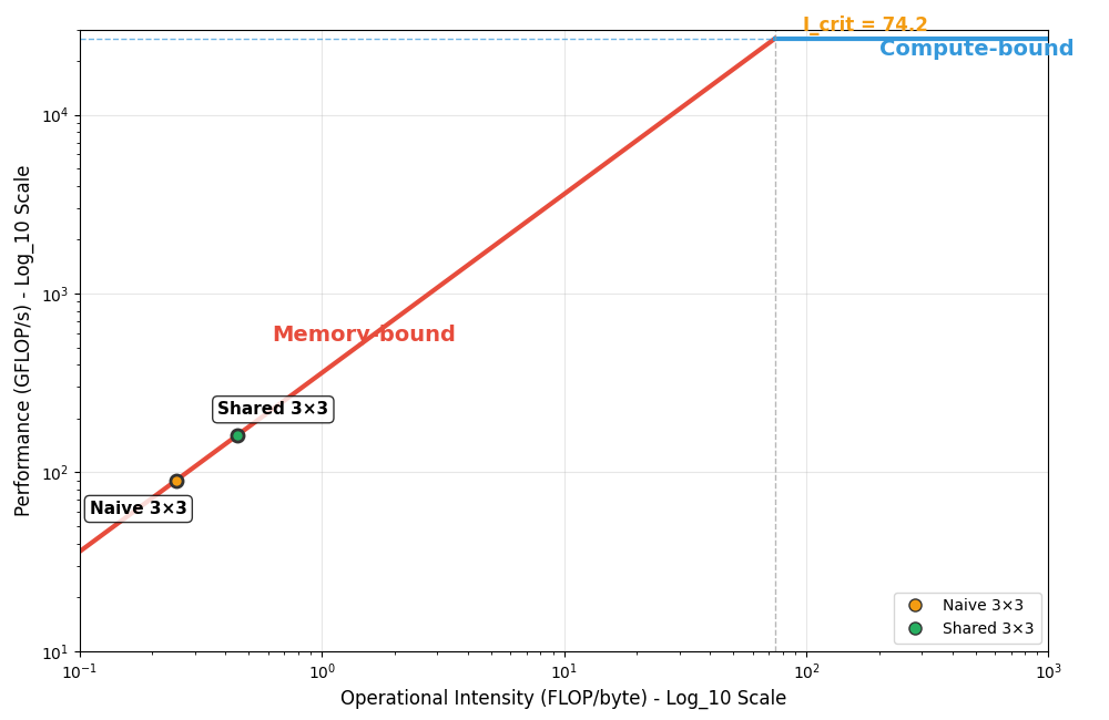
Roofline Estimation
Let’s apply the roofline model to a 3×3 matrix multiplication, which is still small enough to hand-calculate.
The RTX 4000 Ada provides[14]:
- Peak compute: 26.7 TFLOPS (single-precision)
- Peak DRAM bandwidth: 360 GB/s
- Critical intensity: \(I_{crit} = \frac{26.7 \times 10^{12}}{360 \times 10^9} = 74.2\) FLOP/byte
Naive MatMul Analysis
For \(C = A \times B\) where all matrices are 3×3:
Compute work
- Each output element is a dot product of length 3
- 3 fused multiply-adds -> 3 FLOPs per output element
- 9 elements -> 27 FLOPs total
DRAM traffic
- Load matrix A: 9 floats × 4 bytes = 36 bytes
- Load matrix B: 9 floats × 4 bytes = 36 bytes
- Store matrix C: 9 floats × 4 bytes = 36 bytes
- Total: 108 bytes
Operational intensity:
\[I_{naive} = \frac{27 \text{ FLOPs}}{108 \text{ bytes}} = 0.25 \text{ FLOP/byte}\]
Since \(I_{naive} = 0.25 \ll I_{crit} = 74.2\), this kernel is memory-bound.
Predicted performance
\[ \begin{aligned} P_{naive} \;\; & = \min(26.7~\text{TFLOPS},\; 0.25 \times 360~\text{GB/s}) \\ & = \min(26.7~\text{TFLOPS},\; 90~\text{GFLOPS}) \\ & = \boxed{90~\text{GFLOPS}} \end{aligned} \]
Shared Memory Optimization
By staging 3×3 tiles of A and B in shared memory, each element feeds all three required dot products instead of being fetched repeatedly from DRAM.
Improved traffic pattern
- DRAM loads for A and B drop by ~3×
- Stores remain unchanged (36 bytes)
- Approximate traffic: \((36+36)/3 + 36 = 60\) bytes
New operational intensity
\[I_{shared} = \frac{27 \text{ FLOPs}}{60 \text{ bytes}} = 0.45 \text{ FLOP/byte}\]
Predicted performance
\[ \begin{aligned} P_{shared} \;\; & = \min(26.7~\text{TFLOPS},\; 0.45 \times 360~\text{GB/s}) \\ & = \min(26.7~\text{TFLOPS},\; 162~\text{GFLOPS}) \\ & = \boxed{162~\text{GFLOPS}} \end{aligned} \]
This gives us a 1.8× speedup from shared memory optimization, but we’re still memory-bound.
Plot Code
roofline_plot.py
# /// script
# dependencies = [
#   "matplotlib",
#   "numpy",
# ]
# ///

# Run using uv run roofline_plot.py
import matplotlib.pyplot as plt
import numpy as np

peak_compute = 26.7 * 1000  # Convert to GFLOPS
peak_bandwidth = 360  # GB/s
critical_intensity = peak_compute / peak_bandwidth

kernels = [
    {"name": "Naive 3×3", "intensity": 0.25, "performance": 90, "color": "#f39c12"},
    {"name": "Shared 3×3", "intensity": 0.45, "performance": 162, "color": "#27ae60"}
]

def generate_roofline_data():
    # Memory-bound region
    memory_intensities = np.arange(0.01, critical_intensity, 0.05)
    memory_performance = memory_intensities * peak_bandwidth

    # Compute-bound region
    compute_intensities = np.arange(critical_intensity, 1000, 5)
    compute_performance = np.full_like(compute_intensities, peak_compute)

    return memory_intensities, memory_performance, compute_intensities, compute_performance

fig, ax = plt.subplots(figsize=(10, 6.5))

ax.set_xscale('log', base=10)
ax.set_yscale('log', base=10)

mem_i, mem_p, comp_i, comp_p = generate_roofline_data()

ax.loglog(mem_i, mem_p, color="#e74c3c", linewidth=3, label="Memory-bound")
ax.loglog(comp_i, comp_p, color="#3498db", linewidth=3, label="Compute-bound")

ax.axhline(y=peak_compute, color="#3498db", linestyle="--", alpha=0.7, linewidth=1)
ax.axvline(x=critical_intensity, color="#999", linestyle="--", alpha=0.7, linewidth=1)

for kernel in kernels:
    ax.loglog(kernel["intensity"], kernel["performance"],
             'o', color=kernel["color"], markersize=8,
             markeredgecolor="#333", markeredgewidth=2)

    # Add kernel labels with better positioning to avoid overlap
    if kernel["name"] == "Naive 3×3":
        offset_x = kernel["intensity"] * 0.7  # Move left
        offset_y = kernel["performance"] * 0.65  # Move down
    else:  # Shared 3×3
        offset_x = kernel["intensity"] * 1.4  # Move right
        offset_y = kernel["performance"] * 1.3  # Move up

    ax.annotate(kernel["name"],
               (kernel["intensity"], kernel["performance"]),
               xytext=(offset_x, offset_y),
               fontsize=11, fontweight="bold", ha="center",
               bbox=dict(boxstyle="round,pad=0.3", facecolor="white", alpha=0.8))

ax.text(1.5, peak_bandwidth * 1.5, "Memory-bound",
        color="#e74c3c", fontsize=14, fontweight="bold", ha="center")
ax.text(200, peak_compute * 0.8, "Compute-bound",
        color="#3498db", fontsize=14, fontweight="bold")

ax.text(critical_intensity * 1.3, peak_compute * 1.1,
        f"I_crit = {critical_intensity:.1f}",
        color="#f39c12", fontsize=12, fontweight="bold")

ax.set_xlim(0.1, 1000)
ax.set_ylim(10, 30000)
ax.set_xlabel("Operational Intensity (FLOP/byte) - Log_10 Scale", fontsize=12)
ax.set_ylabel("Performance (GFLOP/s) - Log_10 Scale", fontsize=12)
ax.grid(True, alpha=0.3)

legend_elements = [plt.Line2D([0], [0], marker='o', color='w',
                             markerfacecolor=k["color"], markersize=8,
                             label=k["name"], markeredgecolor="#333")
                  for k in kernels]
ax.legend(handles=legend_elements, loc="lower right")

plt.tight_layout()
plt.savefig('./mojo_gpu_puzzles/p14_roofline_naive_and_shared.png', bbox_inches='tight')

print("Performance Analysis:")
print("-" * 40)
for kernel in kernels:
    efficiency = (kernel["performance"] / peak_compute) * 100
    print(f"{kernel['name']}:")
    print(f"  Intensity: {kernel['intensity']} FLOP/byte")
    print(f"  Performance: {kernel['performance']} GFLOP/s")
    print(f"  Efficiency: {efficiency:.1f}% of peak")
Key Insights
- Intensity grows with matrix size - For naive \(N \times N\) GEMM: \(I = \frac{N^3}{4N^2} = \frac{N}{4}\) FLOP/byte
- Small kernels are bandwidth-bound - Even perfect caching can’t reach the 74 FLOP/byte crossover until \(N \approx 300\)
- Shared memory helps, but only up to the ridge - Further speedups require compute-side tuning (tensor cores, ILP, etc.)
Next, we’ll look at one specific optimisation for Matmul: Tile-based GEMM!
Tiled Matrix-Multiplication (GEMM)
Our shared-memory kernel already cut global-DRAM traffic by loading each A[i,k] / B[k,j] element once per thread row/column instead of once per output multiply.
For large matrices, however, even that version still:
- Brings the entire row of
Aand column ofBinto shared SRAM, quickly exhausting the 48–112 KiB available per SM. - Leaves many threads idle while others finish their portion of the dot-product.
- Misses an opportunity to keep a hot, register-resident accumulator and hide global-latency behind computation.
Enter tiling / blocking — the canonical GPU GEMM strategy.
Tile?
Think of an N×N matmul as a chessboard. Instead of letting every thread wander across the whole board, we slice it into T×T sub-squares (tiles).
A thread-block is assigned one output tile, and:
- Cooperatively loads the matching
T×TA-tile and B-tile from global DRAM to shared memory (two coalesced 2-D memcpy’s). - Performs
Tfused-multiply-add sweeps of that data, each thread keeping its running sum in a register. - Barriers, slides the tile window by
Talong the inner-kdimension, and repeats until the dot-product is complete. - Finally writes the
T×Tblock ofCback to DRAM.
Each element of A/B is now read once per tile - independent of N, and re-used T times, boosting arithmetic intensity from O(1) to O(T) FLOP/B.
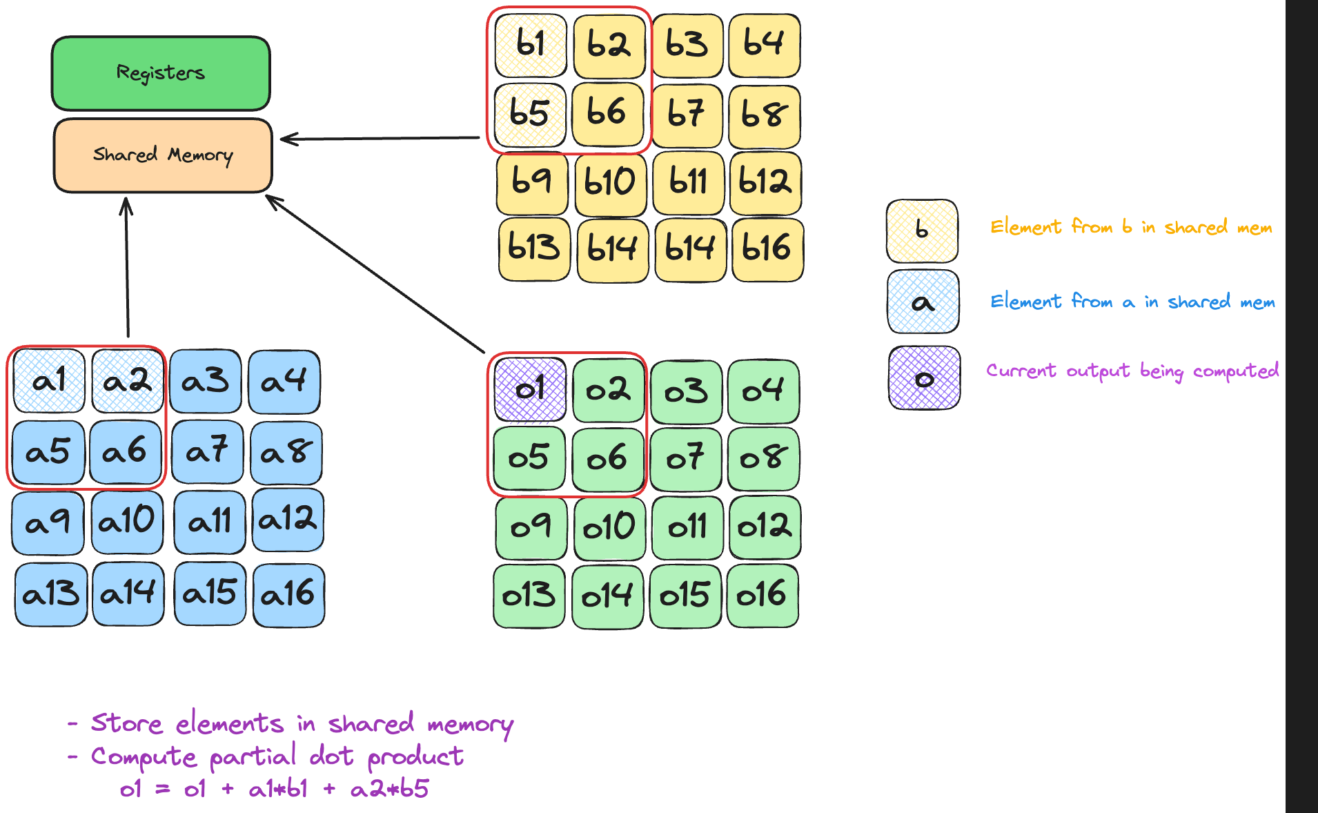
Memory mapping for tiled GEMM
The memory hierachy(discussed in the previous post), is utilised as follows:
- Registers: per-thread accumulators that hold partial
Cvalues across all tile iterations - Shared SRAM: the current
A_tileandB_tile, cooperatively loaded once and reused T times
- Global HBM: original A, B matrices and final C; each element touched once per tile load/store
Raw Memory
Manual Indexing Tiled Matmul
p14_matmul_tiled_manual.mojo
alias SIZE_TILED = 8 # Size of the matrix we are multiplying, NOT the size of a tile
alias BLOCKS_PER_GRID_TILED = (3, 3)  # each block convers 3x3 elements
alias THREADS_PER_BLOCK_TILED = (TPB, TPB)
alias layout_tiled = Layout.row_major(SIZE_TILED, SIZE_TILED)


fn matmul_tiled[
    layout: Layout, size: Int
](
    output: LayoutTensor[mut=False, dtype, layout],
    a: LayoutTensor[mut=False, dtype, layout],
    b: LayoutTensor[mut=False, dtype, layout],
):
    local_row = thread_idx.y
    local_col = thread_idx.x
    global_row = block_idx.y * TPB + local_row
    global_col = block_idx.x * TPB + local_col

    shared_a = tb[dtype]().row_major[TPB, TPB]().shared().alloc()
    shared_b = tb[dtype]().row_major[TPB, TPB]().shared().alloc()

    var local_sum: output.element_type = 0.0

    @parameter
    # (size + TPB - 1) // TPB == ceil(size / TPB) -> number of tile-steps we need
    for tile in range((size + TPB - 1) // TPB):
        # Load elements of A into shared mem
        if global_row < size and (tile * TPB + local_col) < size:
            shared_a[local_row, local_col] = a[
                global_row, tile * TPB + local_col
            ]

        # Load elements of B into shared mem
        if global_col < size and (tile * TPB + local_row) < size:
            shared_b[local_row, local_col] = b[
                tile * TPB + local_row, global_col
            ]

        barrier()

        # Perform matmul
        if global_row < size and global_col < size:

            @parameter
            for k in range(min(TPB, size - tile * TPB)):
                local_sum += shared_a[local_row, k] * shared_b[k, local_col]

            barrier()

        if global_row < size and global_col < size:
            output[global_row, global_col] = local_sum
pixi run p14 --tiled
# out: HostBuffer([2240.0, 2296.0, 2352.0, 2408.0, 2464.0, 2520.0, 2576.0, 2632.0, 5824.0, 6008.0, 6192.0, 6376.0, 6560.0, 6744.0, 6928.0, 7112.0, 9408.0, 9720.0, 10032.0, 10344.0, 10656.0, 10968.0, 11280.0, 11592.0, 12992.0, 13432.0, 13872.0, 14312.0, 14752.0, 15192.0, 15632.0, 16072.0, 16576.0, 17144.0, 17712.0, 18280.0, 18848.0, 19416.0, 19984.0, 20552.0, 20160.0, 20856.0, 21552.0, 22248.0, 22944.0, 23640.0, 24336.0, 25032.0, 23744.0, 24568.0, 25392.0, 26216.0, 27040.0, 27864.0, 28688.0, 29512.0, 27328.0, 28280.0, 29232.0, 30184.0, 31136.0, 32088.0, 33040.0, 33992.0])
# expected: HostBuffer([2240.0, 2296.0, 2352.0, 2408.0, 2464.0, 2520.0, 2576.0, 2632.0, 5824.0, 6008.0, 6192.0, 6376.0, 6560.0, 6744.0, 6928.0, 7112.0, 9408.0, 9720.0, 10032.0, 10344.0, 10656.0, 10968.0, 11280.0, 11592.0, 12992.0, 13432.0, 13872.0, 14312.0, 14752.0, 15192.0, 15632.0, 16072.0, 16576.0, 17144.0, 17712.0, 18280.0, 18848.0, 19416.0, 19984.0, 20552.0, 20160.0, 20856.0, 21552.0, 22248.0, 22944.0, 23640.0, 24336.0, 25032.0, 23744.0, 24568.0, 25392.0, 26216.0, 27040.0, 27864.0, 28688.0, 29512.0, 27328.0, 28280.0, 29232.0, 30184.0, 31136.0, 32088.0, 33040.0, 33992.0])The new formulas in the tiling implementation deserve explanation. Let’s break them down into key concepts:
How many Tiles are needed?
This is the expression: range((size + TPB - 1) // TPB)
The key idea here is: Step through k by TPB each time; if there’s a leftover chunk, do one last tile for it.
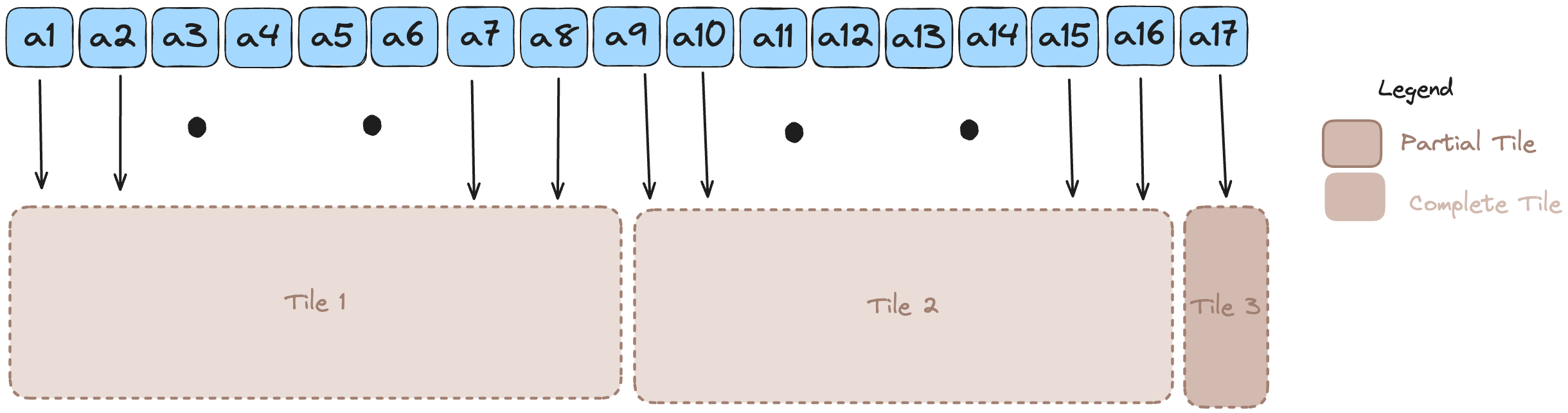
The above example needs 3 tiles. Ceiling division captures this with a simple formula: \[ \lceil\frac{size}{TPB}\rceil = \lfloor\frac{size + TPB - 1}{TPB}\rfloor \]
Which element does a thread fetch in this tile?
Each thread snags two scalars—one from A, one from B.
tile is simply “which chunk of k are we on?”
Inside a block, a thread owns a single output cell C[global_row, global_col]. To finish that cell it must walk k, multiplying aligned pairs (A[row, k], B[k, col]).
On tile t the fetches are
A = a[global_row, t*TPB + local_col]
B = b[t*TPB + local_row, global_col]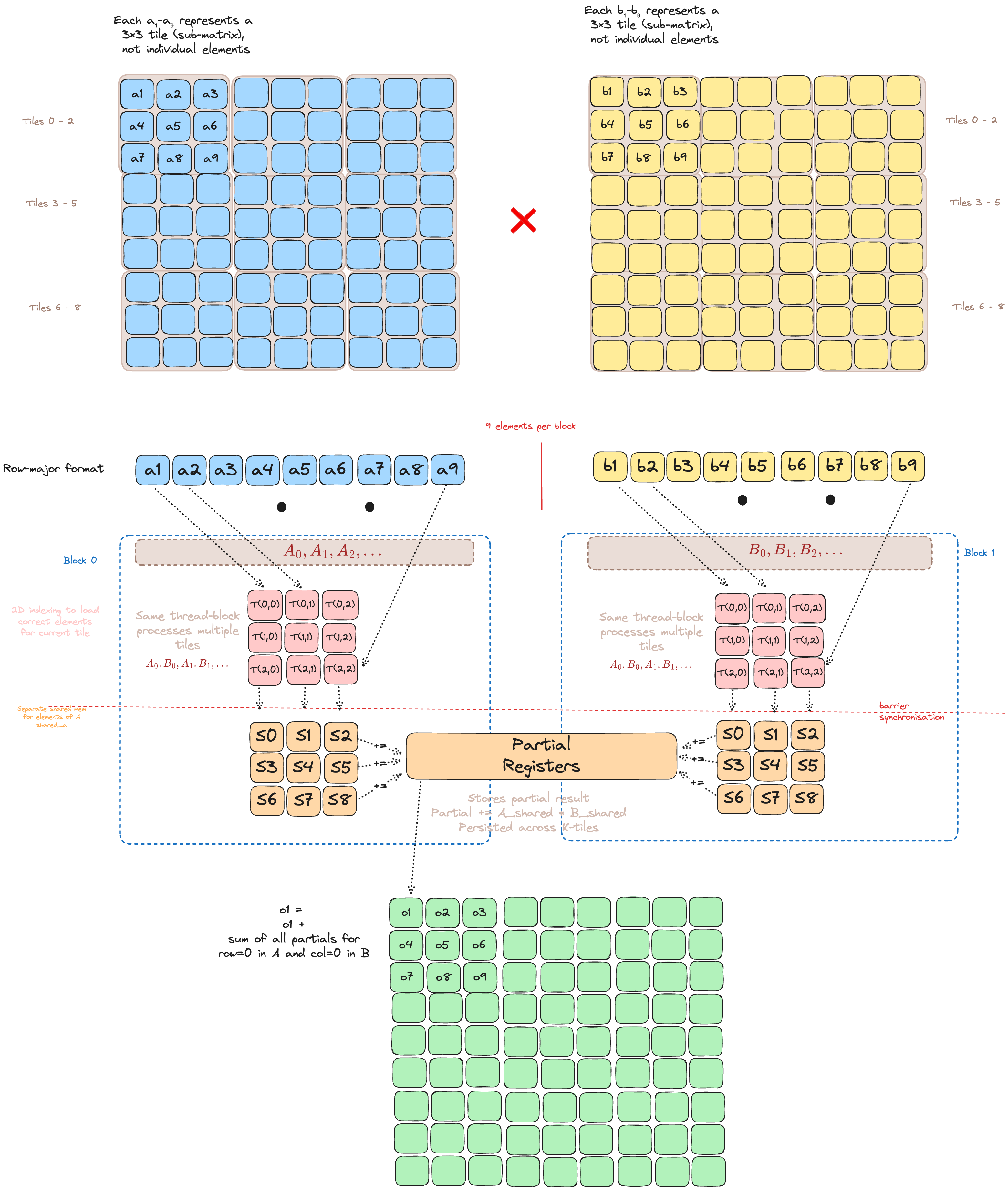
Both reads cover the same k-slice (t*TPB … t*TPB+TPB-1), so every multiply in this round lives entirely in shared memory.
Why do we swap local_row and local_col for B?
GPUs coalesce global memory when adjacent threads read adjacent addresses. With the swap:
- For A: neighboring threads in x-direction (
local_col) read consecutive k’s ⇒ coalesced - For B: neighboring threads in y-direction (
local_row) read consecutive k’s ⇒ also coalesced
Without the swap, one matrix would be fetched “strided” collapsing into 32 separate memory transactions per warp - a 32× slowdown on bandwidth-bound kernels.
Quick primer: Shared memory isn’t one monolithic block. It’s chopped into 32 independent “banks”[15] [16].
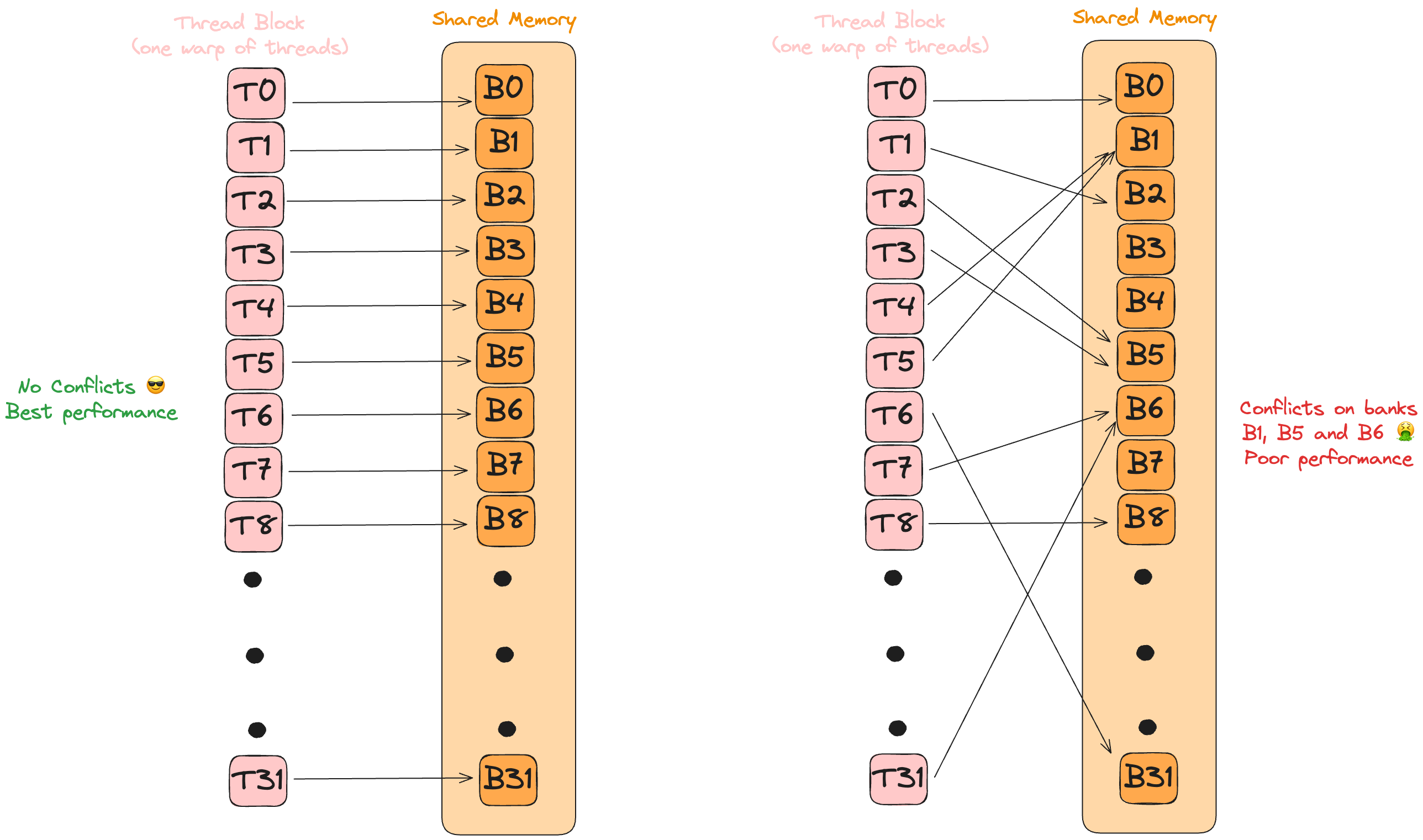
Each is a tiny SRAM with its own read/write port that can service one request (or one 32-bit access per cycle). A warp hits peak bandwidth only when every thread lands in a different bank (or all hit the same address, which hardware can broadcast). If two threads target different addresses inside the same bank during the same cycle, the hardware must serialize them, referred to as a bank conflict.
Beyond coalescing, our tile layout also sidesteps these conflicts. Because b_shared[k, threadIdx.x] maps each thread to a distinct bank (while a_shared[threadIdx.y, k] is broadcast-friendly), all 32 memory ports stay busy with zero serialization.
Choosing the Right Tile Size
While the current puzzle selects \(TPB=3\) with tile size \(TPBxTPB\), choosing the tile size is a balancing act.
Exact numbers vary with GPU, kernel, and precision [[17]][18].
I’m still learning the dark art of GPU perf tuning, so I’ll save the details for a future post once I’ve had more time to experiment.
TLDR: For each tile, we will sync (barrier), compute, shift to next tile, repeat. But this is just the baseline - there’s always a deeper optimization rabbit hole!
LayoutTensor
While the manual tiling approach works, it suffers from indexing complexity that obscures the algorithm’s intent and creates opportunities for bugs. Mojo’s LayoutTensor API provides an elegant solution that maintains performance while dramatically improving code clarity.
The Pain of Manual Indexing
The manual implementation requires careful coordinate arithmetic:
- Nested index calculations like
tile * TPB + local_colthat can easily introduce off-by-one errors - Separate bounds checking for each matrix load operation
- Explicit management of tile boundaries and edge cases
- Code that prioritizes performance over readability
LayoutTensor provides a tile() method that creates zero-copy [7] views into sub-regions of tensors [19]. This eliminates manual indexing gymnastics while keeping identical performance.
A LayoutTensor.tile[tile_height, tile_width](block_row, block_col) call returns a view of the specified tile without copying data, at no cost!
The transformation from manual indexing to LayoutTensor simplifies the loading logic:
# Load elements of A into shared mem
- if global_row < size and (tile * TPB + local_col) < size:
-     shared_a[local_row, local_col] = a[
-         global_row, tile * TPB + local_col
-     ]
-
- # Load elements of B into shared mem
- if global_col < size and (tile * TPB + local_row) < size:
-     shared_b[local_row, local_col] = b[
-         tile * TPB + local_row, global_col
-     ]
# Create tile views (zero-copy)
+ a_tile = a.tile[TPB, TPB](block_idx.y, idx)
+ b_tile = b.tile[TPB, TPB](idx, block_idx.x)

# Asynchronous copy to shared memory
+ copy_dram_to_sram_async[thread_layout=load_a_layout](a_shared, a_tile)
+ copy_dram_to_sram_async[thread_layout=load_b_layout](b_shared, b_tile)

# Synchronize all async copies
+ async_copy_wait_all()
Full solution looks as follows:
LayoutTensor Tiled Matmul
p14_matmul_layout_tensor.mojo
alias SIZE_TILED = 9
alias BLOCKS_PER_GRID_TILED = (3, 3)  # each block covers 3x3 elements
alias THREADS_PER_BLOCK_TILED = (TPB, TPB)
alias layout_tiled = Layout.row_major(SIZE_TILED, SIZE_TILED)


fn matmul_tiled[
    layout: Layout, size: Int
](
    output: LayoutTensor[mut=True, dtype, layout],
    a: LayoutTensor[mut=False, dtype, layout],
    b: LayoutTensor[mut=False, dtype, layout],
):
    # LayoutTensor APIs
    out_tile = output.tile[TPB, TPB](block_idx.y, block_idx.x)
    a_shared = tb[dtype]().row_major[TPB, TPB]().shared().alloc()
    b_shared = tb[dtype]().row_major[TPB, TPB]().shared().alloc()
    local_row = thread_idx.y
    local_col = thread_idx.x

    var local_sum: output.element_type = 0.0

    alias load_a_layout = Layout.row_major[1, TPB]()
    alias load_b_layout = Layout.row_major[TPB, 1]()

    @parameter
    for idx in range((size + TPB - 1) // TPB):
        a_tile = a.tile[TPB, TPB](block_idx.y, idx)
        b_tile = b.tile[TPB, TPB](idx, block_idx.x)

        copy_dram_to_sram_async[thread_layout=load_a_layout](a_shared, a_tile)
        copy_dram_to_sram_async[thread_layout=load_b_layout](b_shared, b_tile)

        async_copy_wait_all()

        @parameter
        for k in range(min(TPB, size - idx * TPB)):
            local_sum += a_shared[local_row, k] * b_shared[k, local_col]

        barrier()

    # Store result after all tiles processed
    if (
        block_idx.y * TPB + local_row < size
        and block_idx.x * TPB + local_col < size
    ):
        out_tile[local_row, local_col] = local_sum
Synchronization and Memory Hierarchy
The copy_dram_to_sram_async() function [20] enables asynchronous memory transfers from global to shared memory, while async_copy_wait_all() [21] provides a synchronization barrier that ensures all pending transfers complete before computation proceeds.
This pattern allows the GPU to:
- Overlap memory transfers with other computations using dedicated copy engines
- Utilize specialized hardware for efficient data movement
- Maintain correct execution ordering across thread blocks
- Bypass intermediate registers for improved memory hierarchy efficiency
Important: async_copy_wait_all() only synchronizes the asynchronous copy operations—threads still need explicit barriers (barrier()) to ensure all threads in a block see the shared memory data before computation begins.
Conclusion
Across these puzzles, we’ve implemented the four fundamental archetypes that power most GPU computing:
| Pattern | Puzzles | Core Technique |
|---|---|---|
| Map-Reduce | dot product, axis-sum | warp-level parallel reduction trees |
| Stencil | pooling, 1D/2D convolution | spatial tiling with halo exchanges |
| Scan | prefix sum | hierarchical up-sweep + down-sweep |
| Dense Linear Algebra | matrix multiplication | cooperative tiling + register reuse |
These four archetypes form the building blocks for complex ML kernels, each with specific memory access patterns and synchronization strategies.
Next up: Moar GPU kernels, and finally tackling our favorite technique for the past few years: Attention!
Thanks for sticking around! I hope you picked up a trick or two! Spotted a bug or have a sharper optimization? Open an issue in the repo, or ping me on Twitter/X. Happy hacking!
References
@parameter) in mojo.” 2025. Available: https://docs.modular.com/mojo/manual/decorators/parameter/#parametric-closure